HANA database partitioning

1. Introduction

The partitioning feature of the SAP HANA database splits column-store tables horizontally into disjunctive sub-tables or partitions. In this way, large tables can be broken down into smaller, more manageable parts.

Partitioning is only available for tables located in the column store. The row store does not support partitioning.

BW systems are handled separately, please refer to chapter “BW Systems”.

1.1 Reasons and background of partitioning

Following are some of the reasons, next to the advantages described later, to perform partitioning:

In SAP HANA, a non-partitioned column store tables can’t store more than 2 billion rows.
Large table / partition sizes in column store are mainly critical with respect to table optimizations like delta merges and optimize compressions (SAP Notes 2057046 – FAQ: SAP HANA Delta Merges, 2112604 – FAQ: SAP HANA Compression):
- Memory requirements are doubled at the time of the table optimization.
- There is an increased risk of locking issues during table optimization.
- The CPU consumption can be significant, particularly during optimize compression runs.
- The I/O write load for savepoints is significant and can lead to trouble like a long critical phase (SAP Note 2100009 – FAQ: SAP HANA Savepoints)
SAP HANA NSE: Range partitions with old data can be offloaded easier.

Therefore you should avoid using particularly large tables and partitions and consider a more granular partitioning instead. A reasonable size threshold is typically 50 GB, so it can be useful to use a more granular partitioning in case this limit is exceeded.

1.2 Best Practices

The following best practices should be kept in mind:

Keep the number of partitioned tables low
Keep the number of partitions per table low (maximum 8 partitions)
Maximum 100 – 200 million rows per partition (recommended).
Define partitioning on as few columns as possible
For SAP Suite on HANA, keep all partitions on same host
Repartitioning rules: When repartitioning, choose the new number of partitions as a multiple or divider of current number of partitions.
Avoid unique constraints
Throughput time: 10-100 G/hour

HASH partitioning on a selective column being part of the primary key; check which sorting option is used mostly.

1.3 Advantages

These are some advantages of partitioning:

Load Balancing: In a distributed system. Individual partition can be distributed across multiple Hosts.
Record count: Storing more than 2 billion rows in a table.
Parallelization: Operations can be parallelized by using several execution threads.
Partition Pruning: Queries are analyzed to see if they match the given partitioning specification of a table (STATIC) or the content of specific columns in aging tables (DYNAMIC).
Remark: When a table is range partitioned based on MONTH and in the WHERE clause YEAR is selected, all partitions are scanned and not only the 12 partitions belonging to the year.
Delta merge performance: Only changed partitions must be duplicated in the RAM, instead of the entire table.

1.4 Partitioning Types

The following partioning types can be used, but normally only HASH and RANGE are used:

HASH: Distribute rows to partitions equally for load balancing and to overcome the 2 billion row limitation.
ROUND-ROBIN: Achieve an equal distribution of rows to partitions.
RANGE: Dedicated partitions for certain values or value ranges in a table.
Multi-level (HASH/RANGE) First partition on level 1, than on level 2.

1.5 Parameters

The following optional parameters can be set to optimize HANA partitioning, if required.

Inifile	Section	Parameter	Value	Remark
indexserver.ini	joins	single_thread_execution_for_partitioned_tables	false	Allow parallelization
indexserver.ini	partitioning	split_threads	<number>	Parallelization number for repartitioning; 80 % of max_concurrency
indexserver.ini	table_consistency_check	check_repartitioning_consistency	true	Implicit consistency check

SQL commands:

ALTER SYSTEM ALTER CONFIGURATION ('indexserver.ini','SYSTEM') SET ('joins',' single_thread_execution_for_partitioned_tables') = 'false' WITH RECONFIGURE;

ALTER SYSTEM ALTER CONFIGURATION ('indexserver.ini','SYSTEM') SET ('partitioning','split_threads') = '<number>' WITH RECONFIGURE;

ALTER SYSTEM ALTER CONFIGURATION ('indexserver.ini','SYSTEM') SET ('table_consistency_check','check_repartitioning_consistency') = 'true' WITH RECONFIGURE;

1.6 Privileges

The following privileges should be granted to the user executing the partitioning:

System privilege: PARTITION_ADMIN

For the user examining the partitioning, the following privilege might also be of interest:

SELECT on schema

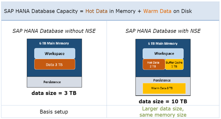
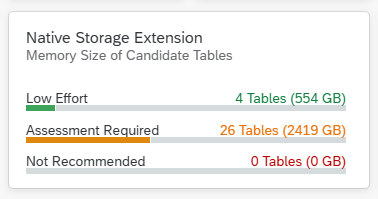
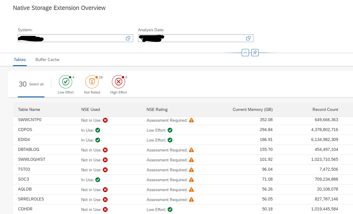
1.7 Remark on partitioning for NSE

Whenever a table is queried and if that table or partition is not present in memory HANA automatically loads it into the memory either partially or fully.

If that table is partitioned, which ever row that is getting queried, then that specific partition which has the required data gets into memory.

Even if you only need 1 row from a partition of a table which has 1 billion records, that entire partition will get loaded either partially or fully.

In HANA we can never load 1 row alone into memory from a table.

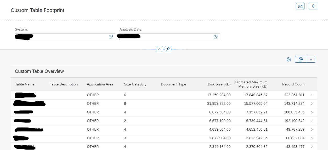
2. Determine candidates

Check which tables are larger than 50G or have more than 1 billion records:

select a.table_name, (select string_agg(column_name,', ') from index_columns where constraint = 'PRIMARY KEY' and table_name = a.table_name group by table_name) "Primary Key Columns",

case a.is_partitioned

when 'TRUE'

then (select LEVEL_1_TYPE || '(' || replace(LEVEL_1_EXPRESSION,'"','') || ')#' || LEVEL_1_COUNT from partitioned_tables where table_name = a.table_name)

else 'No'

end as "Current Partitioning",

a.record_count "Rows", to_decimal(a.table_size/1024/1024/1024,2,2) "Size GB"

from m_tables a where a.IS_COLUMN_TABLE = 'TRUE'

and (a.record_count > 1000000000 or a.table_size/1024/1024/1024 > 50)

order by a.table_name;

The output will display:

TABLE_NAME: Name of the table
Primary Key Columns: The columns on which the primary key is created
Current Partitioning: If the table is currently partitioned and the partition type, columns and number of partitions
Rows: Number of records in the table
Size GB: Size of the table in memory

3. Determine Partitioning Strategy

In order to choose an appropriate column for partitioning we need to analyze the table usage in depth.

3.1 Technical Tables

3.1.1 With recommendations

In case you can find exact partitioning recommendation on a specific table please follow the recommendation. Check SAP Note 2044468 – FAQ: SAP HANA Partitioning to find the latest information. Here only the most common tables are listed.

Note: Be aware that for tables making use of Data Aging (SAP Note 2416490 FAQ: SAP HANA Data Aging in SAP S/4HANA) or NSE (SAP Note 2799997 FAQ: SAP HANA Native Storage Extension (NSE)) there are certain limitations related to partitioning and so the simple standard approach isn’t possible.

Table Name	Partition Type	Partition Column(s)	Remark
/1CADMC/<id>	HASH	IUUC_SEQUENCE
ACDOCA	HASH	BELNR	if data volume is limited, otherwise see SAP Note 2289491 Best Practices for Partitioning of Finance Tables
ADRC, ADRU	HASH	ADDRNUMBER
AFFV	HASH	AUFPL
AUSP	HASH	OBJEK
BALDAT	HASH	LOG_HANDLE
BDSCONT10, DMS_CONT1_CD1, SBCMCONT1	HASH	PHIO_ID
BKPF, BSEG, BSIS	HASH	BELNR
CDHDR, CDPOS	HASH	OBJECTID, CHANGENR or TABKEY	Use column with best value distribution and use same column for both tables if possible, in some cases OBJECTID for CDHDR and CHANGENR for CDPOS can be the best solution
CKMLCR, CKMLKEPH	HASH	KALNR
COBK, COEP	HASH	BELNR
COFV	HASH	CRID
DBTABLOG	HASH	LOGID
EDID4, EDIDS	HASH	DOCNUM
EQKT	HASH	EQUNR
IDOCREL	HASH	ROLE_A or ROLE_B	The column with better value distribution
JCDS, JEST	HASH	OBJNR
JVTLFZUO	HASH	VBELN
KEPH	HASH	KALNR
KONV	HASH	KNUMV
MATDOC	HASH	MBLNR
MBEW, MBEWH, MVER, MYMFT	HASH	MATNR
MSEG	HASH	MBLNR
PCL2, PCL4	HASH	SRTFD
RESB	HASH	RSNUM
RSEG	HASH	BELNR
SOC3	HASH	SRTFD
SRRELROLES	HASH	OBJKEY
STXL	HASH	TDNAME
SWWCNTP0, SWWLOGHIST	HASH	WI_ID
VBFA	HASH	SoH: VBELV S/4HANA: RUUID

3.1.2 Without recommendations

If there is no specific recommendation for partitioning a table by SAP (e.g. because this is not listed (2044468 FAQ: SAP HANA Partitioning) or the table is a customer specific table) please follow the approach as described in chapter “3.3 Other tables”.

3.2 Finance Tables

There are some recommendation in SAP Note 2289491 Best Practices for Partitioning of Finance Tables for finance tables. Please find some of them below:

Table Name	Partition Type	Partition Column(s)	Remarks
ACDOCA	RANGE	FISCYEARPER
FAGLFLEXA (n/a for S4/HANA)	RANGE	RYEAR	If data volume is not significantly above 1 billion records per year
	RANGE	RBUKRS	Only if there is a reasonable data distribution by company code and the expected data volume of the largest company code is not significantly above 1 billion records
	HASH	DOCNR	If none of the above is possible
BSEGBSE_CLR	HASH	BELNR BELNR_CLR	Try to keep BSEG as small as possible by summarization or other options, e.g. described in note 2591291 FAQ S/4HANA: Error F5 727 when posting via Accounting Interface.
BSIS, BSAS, BSID, BSAD, BSIK, BSAK (n/a for S4/HANA)	RANGE	BUKRSBELNR	If partitioning by company code not reasonable or possible
FAGL_SPLINFO, FAGL_SPLINFO_VAL	HASH	BELNR
ACCTIT, ACCTHD, ACCTCR	HASH	AWREF	Only if SAP Note 178476 High increase of table ACCTIT, ACCTHD or ACCTCR is not applicable

3.3 Other tables

3.3.1 Check with functional teams

Check with the functional team(s).

Ask them which column(s) they query frequently and which column is always part of the where clause .

If they are not very clear on the same we can help them with the plan cache data.

3.3.2 Check M_SQL_PLAN_CACHE

With the help of below query we can get a list of queries that are to identify the where clause:

select top 10 upper(SUBSTR_AFTER(STATEMENT_STRING, 'WHERE')), EXECUTION_COUNT, TOTAL_EXECUTION_TIME

from M_SQL_PLAN_CACHE

where STATEMENT_STRING like '%TABLE%'

and not STATEMENT_STRING like 'select upper(SUBSTR_AFTER(STATEMENT_STRING%'

and not upper(SUBSTR_AFTER(STATEMENT_STRING, 'WHERE')) like ''

and not upper(SUBSTR_AFTER(STATEMENT_STRING, 'WHERE')) like '%UNION%'

and TOTAL_EXECUTION_TIME > 0 and EXECUTION_COUNT > 5

order by TOTAL_EXECUTION_TIME desc;

From the result you have to analyze the where clause and find a common pattern.

Let’s assume that table CDPOS is accessed mostly via MANDT and CHANGENR (This is by the way the case in many SAP customer systems), the solution would be to implement range-range multi-level partitioning for column MANDT (level 1) and column CHANGENR (level 2).

For sure some SQL statements will have to look into several partitions of one MANDT when CHANGENR is not used in the where-clause.

3.3.3 Join Statistics

Check the columns that are getting joined on this table. Use SQL script HANA_SQL_Statistics_JoinStatistics_1.00.120+ from OSS note 1969700 – SQL Statement Collection for SAP HANA and modify the SQL like below.

( SELECT /* Modification section */

      '1000/10/18 07:58:00' BEGIN_TIME,                  /* YYYY/MM/DD HH24:MI:SS timestamp, C, C-S<seconds>, C-M<minutes>, C-H<hours>, C-D<days>, C-W<weeks>, E-S<seconds>, E-M<minutes>, E-H<hours>, E-D<days>, E-W<weeks>, MIN */

      '9999/10/18 08:05:00' END_TIME,                    /* YYYY/MM/DD HH24:MI:SS timestamp, C, C-S<seconds>, C-M<minutes>, C-H<hours>, C-D<days>, C-W<weeks>, B+S<seconds>, B+M<minutes>, B+H<hours>, B+D<days>, B+W<weeks>, MAX */

      'SERVER' TIMEZONE,                              /* SERVER, UTC */
      '%' HOST,
      '%' PORT,
      '<SAP Schema>' SCHEMA_NAME,
      '<TABLE_NAME>' TABLE_NAME,
      '%' COLUMN_NAME,
      'TABLE' ORDER_BY            /* TABLE, REFRESH_TIME, MEMORY */
    FROM
      DUMMY

From the output, you can determine on which column joins are happening most and hence a HASH on this column will make the query runtime faster.

3.3.4 Enable SQL Trace

Enable SQL trace for specific table.

3.3.5 No specific range values

When there is no specific range values that are frequently queried and there is a case like most of the columns are used most of the times, a HASH algorithm will be a best fit.

It is similar to round robin partition, but data will be distributed according to the hash algorithm on their one or two designated primary key columns:

A Hash algorithm can only happen on a PRIMARY key field.
Do NOT choose more than 2 primary key field for HASH
Within the primary key, check for which row has maximum distinct records. That specific column can be chosen for re-partition.

To determine which primary key column can be chosen for re-partitioning, perform below steps.

Load the table fully into memory:
LOAD TABLE ALL;
Select the Primary Key columns and the distinct records per column:
select a.column_name, sum(b.distinct_count)from index_columns a, m_cs_columns bwhere a.table_name = 'TABLE'and a.constraint = 'PRIMARY KEY'and a.table_name = b.table_nameand a.column_name = b.column_namegroup by a.column_nameorder by sum(b.distinct_count) desc;

3.3.6 NSE-based partitioning

Check if there is a column with a date-like format in the primary key. It might be a candidate for NSE based partitioning.

`select distinct a.COLUMN_NAME, a.DATA_TYPE_NAME, a.LENGTH, a.DEFAULT_VALUEfrom TABLE_COLUMNS a, INDEX_COLUMNS bwhere a.TABLE_NAME = b.TABLE_NAMEand a.COLUMN_NAME = b.COLUMN_NAMEand replace(a.DEFAULT_VALUE,'0','') = ''and length(a.DEFAULT_VALUE) >= 4and not a.DEFAULT_VALUE = ''and a.LENGTH between 4 and 14and b.CONSTRAINT = 'PRIMARY KEY'and a.TABLE_NAME = 'TABLE';`

This query only gives an indication. To be sure, query the table itself.

Run the following query and execute the output as the schema owner:

`select 'select top 5 ' \|\| string_agg(COLUMN_NAME,', ') \|\| ' from ' \|\| TABLE_NAME \|\| ';'from INDEX_COLUMNS where CONSTRAINT = 'PRIMARY KEY' and TABLE_NAME = 'TABLE' group by TABLE_NAME`

Output looks like:

select top 5 MANDT, KALNR, BDATJ, POPER, UNTPER from CKMLPP;

Execute the output-query and the result looks like:

MANDT,KALNR,BDATJ,POPER,UNTPER

"100","000117445808","2016","012","000"

"100","000101228530","2016","012","000"

"100","000112967972","2016","012","000"

"100","000112967974","2016","012","000"

"100","000101253542","2016","012","000"

In this case the columns BDATJ contains the YEAR and column POPER contains the MONTH.

Another example might be table DBTABLOG:

select top 5 distinct LOGDATE, LOGTIME, LOGID from DBTABLOG;

Execute the output-query and the result looks like:

LOGDATE,LOGTIME,LOGID

"20200522","225740","721651"

"20200522","114541","061031"

"20200522","114541","063115"

"20200522","114541","064398"

"20200522","114541","065345"

In this case column LOGDATA contains a date format, but we need to convert this to the YEAR. This can be done by dividing LOGDATA by 10000 (from 8 characters to 4 character).

4. Determine Partitions

4.1 Ranges

In case of RANGE partitioning, to get an indication of the number of partitions and the number of rows per partition, execute the queries as mentioned in below chapters, depending on the column value that can be used.

Eventually some partition ranges can be combined.

The ranges (start and end), the number of records and the estimated size per partition will be displayed.

Note: these queries should be executed by the SAP Schema user!

4.1.2 Range on part of column

When a part of column can be used, the value has to be divided by the number of characters you want to remove.

This is the case when you want to use the YEAR from a string that contains YEAR, MONTH, DAY and TIME.

Note: Edit the query with the correct TABLE, with the chosen COLUMN and if required change the divider number. For example, if you want to remove 4 characters from the column, devide by 10000 (1 with 4 zeroes).

Example:

From 8 to 4 characters: divide by 10000 (4 zeroes)
From 8 to 6 characters: divide by 100 (2 zeroes)

Query:

select "Start", "End", "Rows", to_decimal("Est_Size_Gb"*"Rows"/1024/1024/1024,2,2) "Est_Size_GB" from (select to_decimal(COLUMN/RANGE,1,0)*RANGE "Start", to_decimal(COLUMN/RANGE,1,0)*RANGE+RANGE "End", count(*) "Rows", (select table_size/record_count from m_tables where table_name = 'TABLE') "Est_Size_Gb"

from TABLE

group by to_decimal(COLUMN/RANGE,1,0)*RANGE

order by to_decimal(COLUMN/RANGE,1,0)*RANGE);

4.1.2 Range on entire column

The entire column value can be used as a partition.

This is the case when you want to use the YEAR from a string that equals the YEAR.

Query:

`select "Start", "Rows", to_decimal("Est_Size_Gb""Rows"/1024/1024/1024,2,2) "Est_Size_GB"from (select COLUMN "Start", count() "Rows", (select table_size/record_count from m_tables where table_name = 'TABLE') "Est_Size_Gb"from TABLEgroup by COLUMNorder by COLUMN);`

4.2 Determine number of partitions

In case of HASH partitioning, the number of partitions has to be determined.

A good sizing method is:

Keep the number of partitions per table low (maximum 8 partitions)
Maximum 100 – 200 million rows per partition (recommended).
This can be done with the following command.

The number of partitions can be determined with the following query, based on the number of records in the table, divided by 100 million (when too many partitions (> 8), divide by a higher value) or the size of the table in GB devided by 50:

`select to_decimal(round(RECORD_COUNT/100000000,0,round_up),1,0) PART_ON_ROWS,` `to_decimal(round(table_size/1024/1024/1024/50,0,round_up),1,0) PART_ON_SIZE` `from m_tables where TABLE_NAME = 'TABLE';`

5 Implementation

5.1 SQL Commands

The following commands can be used to perform the actual partitioning of tables:

Action	SQL Command
HASH Partitioning	`ALTER TABLE TABLE PARTITION BY HASH (COLUMN) PARTITIONS X;`
ROUND-ROBIN Partitioning	`ALTER TABLE TABLE PARTITION ROUNDROBIN X;`
RANGE Partitioning On part of column	`ALTER TABLE TABLE PARTITION BY RANGE (COLUMN)(PARTITION 0 <= VALUES < 1000,PARTITION XXX <= VALUES < YYY,PARTITION OTHERS);`
RANGE Partitioning On full column	`ALTER TABLE TABLE PARTITION BY RANGE (COLUMN)(PARTITION VALUE = 1000, PARTITION VALUE = 2000, …, PARTITION OTHERS);`
Multi-level (HASH/RANGE) Partitioning	`ALTER TABLE TABLE PARTITION BY HASH (COLUMN1) PARTITIONS X,` `RANGE (COLUMN2) (PARTITION 0 <= VALUES < 1000, PARTITION XXX <= VALUES < YYY, PARTITION OTHERS);`
Move partitions to other servers	`ALTER TABLE TABLE MOVE PARTITION X TO 'server_name:3nn03' PHYSICAL;`
Add new RANGE to existing partioned table On part of column	`ALTER TABLE TABLE ADD PARTITION XXX <= VALUE < YYY;`
Add new RANGE to existing partioned table On full column	`ALTER TABLE TABLE ADD PARTITION VALUE = YYY;`
Drop existing RANGE	`ALTER TABLE TABLE DROP PARTITION XXX <= VALUE < YYY;`
Adjust partitioning type	`ALTER TABLE TABLE PARTITION …`
Delete partitioning	`ALTER TABLE TABLE MERGE PARTITIONS;`

5.2 Automatic new partitions

There is an automatic way to add new partitions besides dynamic range partitioning by record threshold. Starting with SPS06 there is a new interval option for range partitions.

When a new dynamic partition is required, SAP HANA renames the existing OTHER partition appropriately and creates a new empty partition.

Thus, no data needs to be moved and the process of dynamically adding a partition is very quick.

With this feature you can use the following parameters to automatize the split of the dynamic partition based on the number of records.

Inifile	Section	Parameter	Default	Unit	Remark
indexserver.ini	partitioning	dynamic_range_default_threshold	10000000	rows	automatic split once reached row threshold
Indexserver.ini	partitioning	dynamic_range_check_time_interval_sec	900	sec	how often the threshold check is performed

Note: These threshold can be changed to meet the requirements. It can also be set per table, with: ALTER TABLE T PARTITION OTHERS DYNAMIC THRESHOLD 500000;

The partitioning columns need to be dates or numbers.
Dynamic interval is only supported when the partition column type is TINYINT, SMALLINT, INT, BIGINT, DATE, SECONDDATE or LONGDATE.
If no <interval_type> is specified, INT is used implicitly.

To check the DATA_TYPE of the selected column, execute the following query:

`select COLUMN_NAME, DATA_TYPE_NAME, LENGTHfrom TABLE_COLUMNSwhere TABLE_NAME = 'TABLE'and COLUMN_NAME = 'COLUMN';`

Examples:

Action	SQL Command
Quarterly new partition	`ALTER TABLE TABLE PARTITION OTHERS DYNAMIC INTERVAL 3 MONTH;`
Half yearly new partition	`ALTER TABLE TABLE PARTITION OTHERS DYNAMIC INTERVAL 6 MONTH;`
After 2 years new partition	`ALTER TABLE TABLE PARTITION OTHERS DYNAMIC INTERVAL 2 YEAR;`

5.3 Check Progress

To check the overall progress of a running partitioning execution, run the following query:

`select 'Overall Progress: ' \|\| to_decimal(sum(CURRENT_PROGRESS)/sum(MAX_PROGRESS)*100,2,2) \|\| '%'from M_JOB_PROGRESSwhere JOB_NAME = 'Re-partitioning'and OBJECT_NAME like 'TABLE%';`

To check the progress in more detail, run:

`select TO_NVARCHAR(START_TIME,'YYYY-MM-DD HH24:MI:SS') START_TIME,` `to_decimal(CURRENT_PROGRESS/MAX_PROGRESS*100,3,2) \|\| '%' "PROGRESS%",` `OBJECT_NAME, PROGRESS_DETAILfrom M_JOB_PROGRESSwhere JOB_NAME = 'Re-partitioning'and OBJECT_NAME like 'TABLE%';`

6 Aftercare

6.1 HASH Partitioning

For HASH Partitioning, regularly check the number of records per partition and consider repartitioning.

When repartitioning, choose the new number of partitions as a multiple or divider of current number of partitions.

6.2 RANGE Partitioning

For tables with RANGE partitioning, new partitions should be created regularly, when a new range is reached.

Old partitions which are not required anymore, can be dropped.

Next to that, checks need to be performed that not too many rows reside in the OTHERS partition.

To review if new partitions should be added to existing partitioned tables and if records are present in the “OTHERS” partition, execute the following query:

select a.table_name, replace(b.LEVEL_1_EXPRESSION,'"','') "Column", b.LEVEL_1_COUNT "Partitions",

max(c.LEVEL_1_RANGE_MIN_VALUE) "Last_Range_From",

CASE max(c.LEVEL_1_RANGE_MAX_VALUE) WHEN max(c.LEVEL_1_RANGE_MIN_VALUE) THEN 'N/A' ELSE max(c.LEVEL_1_RANGE_MAX_VALUE) END "Last_Range_To",

(select record_count from m_cs_tables where part_id = b.LEVEL_1_COUNT and table_name = a.table_name) "Rows in OTHERS"

from m_tables a, partitioned_tables b, table_partitions c

where a.IS_COLUMN_TABLE = 'TRUE'

and a.is_partitioned = 'TRUE'

and b.level_1_type = 'RANGE'

and a.table_name = b.table_name

and b.table_name = c.table_name

and b.LEVEL_1_COUNT > 1

group by a.table_name, b.LEVEL_1_EXPRESSION, b.LEVEL_1_COUNT

order by a.table_name;

When the “Last_Range_To” column is a date-like column and the date-like partition is already or almost past, add a new partition.

For the tables that have non-zero values in column “Rows in OTHERS”, run the following check to determine the reason why they are in others and if extra partitions should be added.

Note: Edit the query with the correct TABLE and COLUMN and if required change the divider number. For example, if you want to remove 4 characters from the column, devide by 10000 (1 with 4 zeroes).

Example:

From 8 to 4 characters: divide by 10000 (4 zeroes)
From 8 to 6 characters: divide by 100 (2 zeroes)

select a."Start", a."End", case when b.part_id is not null then to_char(b.part_id) else 'OTHERS' end "Partition"

from (select to_decimal(COLUMM/RANGE,1,0)*RANGE"Start", to_decimal(COLUMM/RANGE,1,0)*RANGE+RANGE "End"

from TABLE

group by to_decimal(COLUMM/RANGE,1,0)*RANGE

order by to_decimal(COLUMM/RANGE,1,0)*RANGE) a

left outer join

(select part_id,

case when level_1_range_min_value <> '' then to_decimal(level_1_range_min_value,1,0) else '0' end "Start",

case when level_1_range_max_value <> '' then to_decimal(level_1_range_max_value,1,0) else '0' end "End"

from table_partitions where table_name = 'TABLE') b

on a."Start" >= b."Start" and a."Start" < b."End";

All these actions can be done with the commands as specified in chapter “5.1 SQL Commands”.

6.3 Partitioning Consistency Check and Repair

Once partitioning has been implemented, some consistency checks can and should be performed regularly.

To ensure consistency for partitioned tables, execute checks and repair statements, if required.

You can call general and data consistency checks for partitioned tables to check, for example, that the partition specification, metadata, and topology are correct.

If any of the tests encounter an issue with a table, the statement returns a row with details on the error. If the result set is empty (no rows returned), no issues were detected.

6.3.2 General check

Checks the consistency among partition specification, metadata and topology:

`CALL CHECK_TABLE_CONSISTENCY('CHECK_PARTITIONING', 'SCHEMA', 'TABLE’);`

6.3.2 Extended check

General check plus check whether all rows are located in correct parts:

`CALL CHECK_TABLE_CONSISTENCY('CHECK_PARTITIONING_DATA', 'SCHEMA', 'TABLE’);`

6.3.2 Dynamic range partitioning check

Check for illegal data in a dynamic range OTHERS partition.

Only sequential numerical data is permitted in such a partition, but a varchar column for example, could include illegal characters.

This check will only work for others partitions which are dynamic range enabled:

`CALL CHECK_TABLE_CONSISTENCY('CHECK_PARTITIONING_DYNAMIC_RANGE', 'SCHEMA', 'TABLE’);`

6.3.4 Repairing rows that are located in incorrect parts

If the extended data check detects that rows are located in incorrect partitions this may be repaired by executing:

`CALL CHECK_TABLE_CONSISTENCY('REPAIR_PARTITIONING_DATA', 'SCHEMA', 'TABLE’);`

7 BW Systems

BW takes care of the partitioning of its tables on its own, manual intervention is usually not required. You mainly have to take care that the table placement configuration is maintained properly (SAP Notes 1908075 SAP BW on SAP HANA: Table Placement and Landscape Redistribution and 2334091 SAP BW/4HANA: Table Placement and Landscape Redistribution ). Table distribution (SAP Note 2143736 FAQ: SAP HANA Table Distribution for BW) will then implement the configuration.

The number of first level partitions depends on number of records in the largest table of the table group respectively the TABLE_PLACEMENT configuration.

Default scenario:

Records	Partitions
< 40 million	1
40 – 120 million	3
120 – 240 million	6
> 240 million	12

7.1 Table Placement and Landscape Redistribution

Please check SAP Note 1908075 – SAP BW on SAP HANA: Table Placement and Landscape Redistribution.

In all SAP BW on SAP HANA systems (single node and scale-out) maintain the table placement rules and the required SAP HANA parameters as follows and explained below.

7.1.1 Determine placement strategy

Extract the file TABLE_PLACEMENT.ZIP from the attachment of SAP Note 1908075 SAP BW on SAP HANA: Table Placement and Landscape Redistribution. According to the following matrix, you can determine the suitable file (or files) and the corresponding folder:

HANA 1.0 SPS12 HANA 2.0	Single node	Scale-out with 1 Index server coordinator + 1 active index server worker node	Scale-out with 1 Index server coordinator + 2 active index server worker nodes	Scale-out with 1 Index server coordinator + 3 or more active index server worker nodes
For systems up to and including 2 TB per node	010 = Single node (up to and including 2 TB)	020 = Scale-out (up to and including 2 TB per node) with 1 coordinator and 1 worker node	030 = Scale-out (up to and including 2 TB per node) with 1 coordinator and 2 worker nodes	040 = Scale-out (up to and including 2 TB per node) with 1 coordinator and 3 or more worker nodes
For systems with more than 2 TB per node	050 = Single node (more than 2 TB)	060 = Scale-out (more than 2 TB per node) with 1 coordinator and 1 worker node	070 = Scale-out (more than 2 TB per node) with 1 coordinator and 2 worker nodes	080 = Scale-out (more than 2 TB per node) with 1 coordinator and 3 or more worker nodes

Notes:

Scale-out configurations with less than two active index server worker nodes are not recommended. If the scale-out system uses <= 2 TB per node. See SAP Note 1702409 for details.
InfoCubes and classic/advanced DataStore Objects in scale-out systems are distributed over all nodes – including the coordinator – if the nodes are provided with more than 2 TB main memory. This optimizes memory usage of all nodes – including the coordinator. If this frequently leads to situations with excessively high CPU load on the coordinator, certain BW objects must be distributed to other nodes to reduce the CPU load.
With SAP HANA 1.0 SPS 12 and SAP HANA 2.0, a table for a BW object can have more partitions at the first level than there are valid locations (hosts) for this table, but only if the main memory of the nodes exceeds 2 TB. This is achieved by setting the parameter ‘max_partitions_limited_by_locations’ to ‘false’. The maximum number of partitions at the first level is limited by the parameter ‘max_partitions’. Its value is set depending on the number of hosts.
Some operations in HANA use parallel processing on partition level. If there are more partitions, it is ensured that the CPU resources on larger HANA servers are used more efficiently. If this frequently leads to situations with excessively high CPU load on some or all HANA nodes, it may be necessary to manually adjust the partitioning rules (for some BW objects) to reduce the CPU load. In this context ‘manually’ means that a customer defined range partitioning at the second level must be adjusted, or additional, BW object-specific table placement rules must be created. Please note that manual changes to the partitioning specification of BW-managed tables at database level (via SQL statements) are not supported.
In scale-out systems with 1.5 or 2 TB per nodeand efficient BW housekeeping, the memory usage on the coordinator may be low because InfoCubes and DataStore Objects are not distributed across all nodes (as is the case for systems with more than 2 TB per node). In this scenario, it is not supported to use the rules for table placement for systems with more than 2 TB per node. Instead, you can check the option of identifying DataStore Objects (advanced)that are used as corporate memory, on which therefore little or no reporting takes place, and placing these objects on the coordinator node. This may be a workaround to make better use of the main memory on the coordinator node without causing a significant increase in the CPU load on the coordinator. DataStore objects (advanced) can be placed on the coordinator node with the aid of object-specific rules for table placement. These customer-specific rules for table placement must be reversed if this causes an overly high memory or CPU load on the coordinator node.

Prerequisites:
- only for scale-out systems with 1.5 or 2 TB per node
- only for DataStore Objects (advanced) not for classic DataStore Objects (due to the different partitioning specifications)
- only for DataStore Objects (advanced) that are used as corporate memory i.e. DataStore Objects (advanced) without activation
- sizing rules as documented in the attachment ‘advanced DataStore objects type corporate memory on coordinator node.sql’ must be respected

7.1.2 Maintain scale-out parameters

In SAP BW on SAP HANA scale-out systems only, maintain the parameters recommended in SAP Note 1958216 for the SAP HANA SPS you use.

In an SAP HANA scale-out system, tables and table partitions are assigned to an indexserver on a particular host when they are created. As the system evolves over time you may need to optimize the location of tables and partitions by running automatic table redistribution.

Different applications require different configuration settings for table redistribution.

For systems running SAP BW on SAP HANA or SAP BW/4HANA – SAP HANA 2.0 SPS 04 and higher:

`ALTER SYSTEM ALTER CONFIGURATION ('indexserver.ini','SYSTEM') SET ('table_redist','balance_by_execution_count') = 'false' WITH RECONFIGURE COMMENT 'See SAP Note 1958216';`

7.1.3 Check Table Classification

Make sure that all BW tables have the correct table classification.

For an existing SAP BW on SAP HANA system, you can check the table classification using the report RSDU_TABLE_CONSISTENCY and correct it if necessary. For information about executing the report, see SAP Note 1937062.

This note provides a file “rsdu_table_consistency_<version>.pdf”.

The report does not available on BW4/HANA systems. Please check the note 2668225 – Report RSDU_TABLE_CONSISTENCY is deprecated with SAP BW/4HANA.

Follow the instructions from the latest pdf file.

During the migration of an SAP BW system via SWPM, the report SMIGR_CREATE_DDL ensures that the correct table classification is set.
Before using one of the two reports, implement the current version of the SAP Notes listed in the to SAP Note 1908075 attached file REQUIRED_CORRECTION_NOTES.XLSX. Filter the list in accordance with your release and Support Package, and implement the notes in the specified sequence using transaction SNOTE.

In a heterogeneous system migration using the Software Provisioning Manager (SWPM), you also have to implement these SAP Notes in the source system before you run the report SMIGR_CREATE_DDL. If you perform the migration using the Database Migration Option (DMO), you do not have to implement the SAP Notes in the source system. Instead, you should implement the SAP Notes in the target system or include a transport with those SAP Notes when the DMO prompts you to do so.

The operation of the report is strongly divided into two parts: Check and Repair, which can’t be combined in a single run!

7.1.3.1 Check tables for inconsistencies

The check for inconsistencies is pure read-only for both HANA and BW.

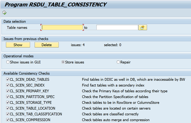
In Tx SE38, run report RSDU_TABLE_CONSISTENCY.

Select “Store issues” and select all checkboxes:

Run the report.

7.1.3.2 Display table consistencies

When you run the report with “Show issues in GUI”, the issues will be displayed.

When you run the report with “Store issues”, the issues will be displayed when executing in foreground.

An example is shown below:

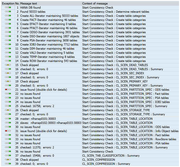
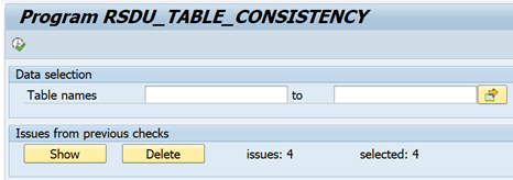
When the report has been executed in the background with option “Store issues”, you can rerun the report and choose “Show”.

The issues only will be displayed:

When you double click on an issue, the details will be displayed:

If you want to repair the issue, select the line and click Save and go back (number of selected items will be displayed):

Please keep I mind, that the displayed columns in the table at different check-scenarios differ. Usually following information will be provided with all scenarios:

Exception: Provides information on the severity of the issue. Red: Inconsistency found or error occurred. There is a need of repair, or failure must be eliminated with further tools Yellow: Warning of unexpected results, but there’s no immediate action needed Green: additional info – no action required
Status: indicates the current state of the issue regarding a possible repair action:
- OK: no error or inconsistency – just info
- REPAIRABLE: this inconsistency should be repairable within RSDU_TABLE_CONSISTENCY
- IRREPARABLE: an inconsistency or an error occurred during the check which can’t be solved within the report. Additional actions or analysis needed to solve this issue
- FAILED: an inconsistency, in which a repair attempt failed. Refer the entry in column ‘Reason’.
- REPAIRED: indicates that the issue was successfully repaired.
Type: shows the type of table like Fact tables, PSA etc.
Reason: This describes the reason why a table is classified as inconsistent. For errors that have occurred during the check, the error text is shown. Some frequently occurring errors are described in section 6 (“Frequently obtained error messages and warnings” at page 14). 5. Table: shown the table name
BW Object: shows the BW Object (InfoCube name, DSO name etc.) the table is liked with.

7.1.3.3 Repair table inconsistencies

A user must first select the issues to be repaired before it can start the repair sequence. Repairing an inconsistence always performs a write action on HANA table properties – the repair will never chance any BW metadata!

Run report RSDU_TABLE_CONSISTENCY again and select repair (with the number of items selected).

Execute the program in background.

Check in SM37 the job log and spool output:

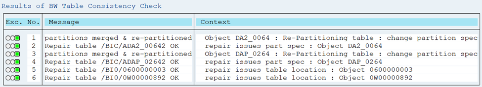
Rerun the check report from chapter “7.1.3.1 Check tables for inconsistencies”. All should be green now!

7.1.4 Perform Database Backup

Perform a full HANA Database backup!

7.1.5 Start Landscape Redistribution

Start the landscape redistribution. Depending on which tool you are using, you will find detailed instructions in the SAP HANA Administration Guide or in the SAP HANA Data Warehousing Foundation – Data Distribution Optimizer.

These actions have to be executed as SYSTEM user in the HANA Tenant DB, preferably from the HANA Studio.

In HANA Studio, go to the Administration Console and select tabs “Landscape” and then “Redistribution”.

Note: These steps can take a long time and should be executed in quiet windows.

7.1.5.1 Save current Table Distribution

Save the current table distribution.

7.1.5.2 Optimize Table Distribution

In the Administration Console, tabs “Landscape” and then “Redistribution”, select the “Optimize Table Distribution” and click Execute. Keep the default settings and click Next. List of the newly, to be implemented, Table Distribution is displayed. Click Execute to start the actual Table Redistribution. The progress can again be followed.

7.1.5.3 Optimize Table Partitioning

In the Administration Console, tabs “Landscape” and then “Redistribution”, select the “Optimize Table Partitioning” and click Execute. Keep the default settings and click Next. A list of the newly, to be implemented, Table Partitioning is displayed. Click Execute to start the actual Table Repartitioning. The progress can again be followed.

9 References

Credits: Rob Kelgtermans

HANA NSE (Native Storage Extension)

1. Introduction

SAP HANA Native Storage Extension (NSE) in a built-in method of SAP HANA, which can be activated and used to offload data to the filesystem, without the need to load it into memory.

The database size can be increased without the need to scale-up or scale-out the database.

All data in the database has a Load Unit property, which defines how data is accessed, loaded and processed by the HANA database.

The data in NSE is “page-loadable”, which means that it is loaded on request by the HANA resource manager into the NSE buffer cache.

The buffer cache manages its own memory pools allocating memory on demand, releasing unused memory and applying smart caching algorithms to avoid redundant I/O operations. A good sizing is important. Too small can lead to Out-Of-Buffer (OOB) events and performance issues. Too large is a waste of memory.

The NSE Advisor is a tool that provides recommendations about load units for tables, partitions or columns. It helps to decide which data should be placed in NSE being page loadable. The required view is “M_CS_NSE_ADVISOR”, which results in a list of tables, partitions and columns with suggestions on whether they should be page or column loadable.

1.1 Reasons

The main reasons for implementing HANA NSE, are:

Reduce HANA memory footprint
Reduce HANA License Costs
Reduce Hardware Costs (no need to Scale-Up or Scale-Out)

1.2 Restrictions

Currently, it is not possible to change the partitioning definition as well as the load unit of a table at once.
First, the table needs to be partitioned using the heterogeneous partitioning definition, afterwards, the load unit can be changed for the whole table or individual partitions.

2. Load Units

There are two types of load units:

Column-loadable: columns are fully loaded into memory when they are used.
Page-loadable: columns are not fully loaded into memory, but only the pages containing parts of the column that are relevant for the query.

The load unit can be defined with CREATE or ALTER statements for tables, partitions or columns.

When not specified, it contains the value “DEFAULT”, which is “column loadable”, but it takes over the value from its parent: Table -> Partition -> Column

Example:

Type	Specified Load Unit	Effective Load Unit
Table	DEFAULT	COLUMN
Partition	Page Loadable	Page Loadable
Column	DEFAULT	Page Loadable

3. Identify WARM data

3.1 Static Approach

Based on these characteristics and some knowledge about your applications you can apply a static approach to identify warm data:

Less-frequently accessed data in your application(s) is e.g. application log-data or statistics data. Their records are often written once and rarely read afterwards.
Less-frequently accessed data is also historical data in the application. Some application tables have e.g. a date/time column that provides an indicator to “split” a table in current and older (historical) parts. This table split can be implemented by a table range-partitioning in the HANA database, where the partition key is e.g., the data/time column in your table.

Without too much knowledge about the applications running on the database, you may also monitor the table access statistics in HANA (m_table_statistics or in the SAP HANA Cockpit) to identify rarely accessed tables.

3.2 Dynamic Approach

This can be achieved with the NSE Advisor.

Since S/4HANA 2021 there are over 150 objects delivered during the EU_IMPORT phase from SAP. The most common once are dictionary tables like DD03L, DOKTL, DYNPSOURCE, TADIR etc. This means every customer with S/4 2021+ will now use NSE. So, please take care of your configuration.

4. Implementation

The NSE implementation contains 3 phases:

Pre-checks
Plan
Execute

4.1 Pre-checks

Before starting, it is wise to perform some checks to define the current situation.

The following SQL commands can be executed in the HANA tenant on which the NSE will be activated:

Used memory

select to_decimal(sum(USED_MEMORY_SIZE)/1024/1024/1024,2,2) "Memory Gb" from M_SERVICE_COMPONENT_MEMORY;

Memory size for tables

select to_decimal(sum(MEMORY_SIZE_IN_TOTAL)/1024/1024/1024,2,2) as "MEM_SIZE_GB" from M_CS_TABLES;

Memory size per component

select COMPONENT, to_decimal(sum(USED_MEMORY_SIZE)/1024/1024/1024,2,2) "Memory Gb" from M_SERVICE_COMPONENT_MEMORY group by COMPONENT order by COMPONENT;

Column store size

select to_decimal(sum(PAGE_SIZE*USED_BLOCK_COUNT)/1024/1024/1024,2,2) as "CS Size GB" from M_DATA_VOLUME_PAGE_STATISTICS where not PAGE_SIZECLASS like '%-RowStore';

4.2 Plan

This phase consist of determining the objects candidates that can be offloaded. There are a few possible options which can/should be combined to come to a proper offload plan.

These are the possible options:

NSE Advisor
Technical and Dictionary Tables
Tables with a low read count
Partitions with low read count
Statistic Server Tables
Audit Log Tables
Partitioning

4.2.1 NSE Advisor

The NSE advisor should only be used either with the HANA Cockpit or the built-in procedure. A mix of both will lead to wrong results.

Use the advisor for representative workloads of your system.

To limit the CPU consumption of the NSE Advisor, set the following parameters:

min_row_count Exclude objects with less than X rows (default: 10000)
min_object_size Ignore objects smaller than X bytes (default: 1048576)

Note: NSE Advisor Recommendations are NOT persistent over a restart!

4.2.1.1 Enable NSE Advisor

Enable via the HANA Cockpit:

Go to the HANA database, select view “All”. In tile “Native Storage Extension”, click in the three dots and choose “Configure NSE Advisor”:

Set the “Enable NSE Advisor” to “ON” and change the “Minimum Object Size” to “1024” MB:

4.2.1.2 Retrieve NSE Advisor recommendations

Generally, the NSE Advisor recommends that you change the load unit of a table, partition, or a column to:

Page-loadable to reduce memory footprint without much performance impact.
Column-loadable to improve performance by keeping hot objects in memory.

The following views can be queried to determine the advices from the NSE Advisor:

M_CS_NSE_ADVISOR

An overview of the objects to be changed:

select * from M_CS_NSE_ADVISOR order by confidence desc;

Same as previous, but in more readable format and only selecting required columns:

select SCHEMA_NAME as SCHEMA, TABLE_NAME, PART_ID, COLUMN_NAME, GRANULARITY as CHANGE_ON, CONFIDENCE,to_decimal(MEMORY_SIZE_IN_MAIN/1024/1024/1024,2,2) as "SIZE_MEM_GB", to_decimal(MAIN_PHYSICAL_SIZE/1024/1024/1024,2,2) as "SIZE_PHYS_GB"from M_CS_NSE_ADVISORwhere not CONFIDENCE = '-1'order by CONFIDENCE desc;

M_CS_NSE_ADVISOR_DETAILS

An overview with more details of all the objects checked:

select * from M_CS_NSE_ADVISOR_DETAILS order by confidence desc;

Same as previous, but in more readable format and only selecting required columns:


select SCHEMA_NAME as SCHEMA, TABLE_NAME, PART_ID, COLUMN_NAME, GRANULARITY as CHANGE_ON,CONFIDENCE, CURRENT_LOAD_UNIT as CHANGE_FROM, TARGET_LOAD_UNIT as CHANGE_TO,to_decimal(MEMORY_SIZE_IN_MAIN/1024/1024/1024,2,2) as "SIZE_MEM_GB",to_decimal(MAIN_PHYSICAL_SIZE/1024/1024/1024,2,2) as "SIZE_PHYS_GB"from M_CS_NSE_ADVISOR_DETAILSwhere not CONFIDENCE = '-1'order by CONFIDENCE desc;

Explanation of the columns:

Column name	Renamed Column	Description
SCHEMA_NAME	SCHEMA	Displays the schema name.
TABLE_NAME		Displays the table name.
COLUMN_NAME		Displays the column name. When the recommendation level is not column, this field is not applicable and the value NULL is used.
PART_ID		Displays the table partition ID. When the recommendation level is not Partition, this field is not applicable, and the value is 0.
CURRENT_LOAD_UNIT	CHANGE_FROM	Displays the current load unit for this object: COLUMN/PAGE.
TARGET_LOAD_UNIT	CHANGE_TO	Displays the recommended load unit for this object: COLUMN/PAGE.
GRANULARITY	CHANGE_ON	Displays the object level at which the recommendation for this table is given: TABLE, PARTITION, or COLUMN.
MEMORY_SIZE_IN_MAIN	SIZE_MEM_GB	Displays the memory consumption size, in bytes, per granularity of the object in main memory. If not LOADED, the value is 0 is used.
MAIN_PHYSICAL_SIZE	SIZE_PHYS_GB	Displays the storage size, in bytes, per granularity of the object.
CONFIDENCE		How sure the NSE advisor is about performing the change.

Note: Columns $trexexternalkey$ or $AWKEY_REFDOC$GJAHR$ are internal columns (SAP Note 2799997 – Q15 “How to handle NSE advisor recommendations to move columns like $trexexternalkey$ or $AWKEY_REFDOC$GJAHR$?”) that refer to the primary key respectively a multi-column index/concat attribute. Indexes can be moved to NSE as well.

Identify index name:

select SCHEMA_NAME, TABLE_NAME, INDEX_NAME, INDEX_TYPE, CONSTRAINT
from INDEXES where TABLE_NAME = '<table_name>';

Change the index load granularity

ALTER INDEX "<schema>"."<index_name>" PAGE LOADABLE;

4.2.1.3 Disable the NSE Advisor

In the same screen as the enable function, now set the “Enable NSE Advisor” to “OFF”.

4.2.2 Technical and Dictionary Tables

Some technical and dictionary tables can be offloaded, as they are not read often and only inserts are being performed.

Examples: Change documents (CDPOS, CDHDR), Application Log (BALDAT), IDocs (EDID4), Table changes (DBTABLOG), Archiving (ZARIX*).

It comes down to the following tables:

CDPOS ^*
CDHDR ^*
BALDAT
EDID4
DBTABLOG
ZARIX%
%~OLD (SAP Note 2198923)

Note: Be careful with CDPOS and CDHDR, as after changing these tables, the NSE advisor gives:

CDHDR should be changed back to COLUMN loadable.
CDPOS should be changed back to COLUMN loadable for columns OBJECTID and CHANGENR

4.2.2.1 Page Preferred versus Page Enforced

Starting SAP S/4HANA 2021, there are tables with ‘paged preferred’ load unit in ABAP Data Dictionary (DDIC):

Run report DD_REPAIR_TABT_DBPROPERTIES for all tables (‘check only’ option) to determine tables having a ABAP DDIC load unit ‘page preferred’ but have actual load unit ‘column’ in the HANA database.

For a quick glance on the load unit settings in DDIC, you may check field LOAD_UNIT in table DD09L:

‘P’= ‘page preferred’, ‘Q’ ‘page enforced’

The following query can be used to determine the table partitions of which the preferred load unit is ‘PAGE’, but the actual load unit is ‘COLUMN’:

select a.SCHEMA_NAME, a.TABNAME, a.LOAD_UNIT, b.LOAD_UNIT, to_decimal(sum(b.MEMORY_SIZE_IN_TOTAL/1024/1024/1024,2,2) "Memory G"from <SAP Schema>.DD09L a, M_CS_TABLES b where a.TABNAME = b.TABLE_NAME and b.LOAD_UNIT = 'COLUMN' and a.LOAD_UNIT = 'P' group by a.TABNAME, a.LOAD_UNIT, b.LOAD_UNIT order by sum(b.MEMORY_SIZE_IN_TOTAL/1024/1024/1024) desc;

For more information, see SAP Note 2973243.

Column Preferred or Page Preferred

Column Preferred is the default behavior.
The load unit is only applied to the database table (runtime object in SAP HANA) upon creation of the table. As a consequence, if the DDIC setting of an existing table that is initially “column loadable” is changed to “page preferred” in a new release of SAP S/4HANA, an upgrade to that release will not change the load unit setting of the database table – the table will remain “column loadable” in SAP HANA.
Changing from one preferred load unit to another does not change the load unit on the database.
The ABAP DDIC consistency check does not consider the load unit. It is accepted if the load unit on the database differs from the values specified in the DDIC.
During a table conversion, the actual NSE settings of the runtime object in the HANA database will be preserved.

Column Enforced or Page Enforced

The load unit is specified upon creation of the table. Furthermore, changes to the load unit in the ABAP DDIC result in corresponding changes on the database.
Changing the enforced load unit results in a corresponding change on the database.
The ABAP DDIC consistency check takes the load unit into account. Different values for the load unit in the DDIC and on the database result in tables that are inconsistent from the DDIC point of view.
For the “Page Enforced” load unit setting, the technical restrictions apply as described in the context of S/4HANA 2020.
For the “Enforced” flavor of load unit settings, the behavior during table conversion is as described in the context of S/4HANA 2020.

4.2.3 Statistics Server Tables

The ESS (embedded statistics server) tables are not part your business workload. They are used for the performance and workload data of the system. This means they are only used for read load when you have some issues and your DBA or SAP is analyzing the system.
These column tables of the SAP HANA statistics server are not using NSE as default. It is recommended to also activate NSE for the column tables of the SAP HANA statistics server.

Determine the current load unit:

select distinct LOAD_UNIT from SYS.TABLES where SCHEMA_NAME = '_SYS_STATISTICS' and IS_COLUMN_TABLE = 'TRUE' and IS_USER_DEFINED_TYPE = 'FALSE';

When the output value is ‘DEFAULT’, activate NSE for column tables of HANA statistics server using PAGE LOADABLE by running the following command with a user with sufficient permissions:

call _SYS_STATISTICS.SHARED_ALTER_PAGE_LOADABLE;

4.2.6 Audit Log Tables

Starting with HANA 2.0 Rev. 70 it is possible to page out the table “CS_AUDIT_LOG_”.

Check the current setting with the following command:

select LOAD_UNIT from SYS.TABLES where SCHEMA_NAME = '_SYS_AUDIT' and TABLE_NAME = 'CS_AUDIT_LOG_';

When the output value is ‘DEFAULT’, activate NSE for the audit log tables with the following command:

ALTER SYSTEM ALTER AUDIT LOG PAGE LOADABLE;

4.2.7 Partitioning

When NSE is used for a table (regardless of whether the full table is page loadable, or only selected columns or partitions), comparatively small partitions should be designed in order to optimize IO-intensive operations such as delta merges. Because of the focus on IO, the relevant measurable is not the number of records per partition, but rather the partition size in bytes. When using NSE with a table, partition sizes should be smaller than 10 GB. This also means that if the size of a table that is fully or partially (selected columns) in NSE reaches 10 GB, this table should be partitioned.

This should be analyzed and tested carefully and depends highly on the usage of the table by your business. Mostly the current and the last year is interesting for most scenarios. This means anything older than 2 years can be paged out. Here you have to choose a partition attribute. Mostly there is a time range attribute like FYEAR or GJAHR. Here you can partition by year / quarter / month. This depends on the amount of data.

Monitoring the buffer hit ratio, fill degree of partitions, performance of SQLs (may be new coding which was not analyzed) and creating new partitions for new months, quarter or years. It is an ongoing process and every new HANA revisions has its own new features.

The following query retrieves partitioned tables with range partitions older than 3 years.

select a.schema_name, a.table_name, c.part_id, replace(b.LEVEL_1_EXPRESSION,'"','') "Column",
max(c.LEVEL_1_RANGE_MIN_VALUE) "Last_Range_From",
max(c.LEVEL_1_RANGE_MAX_VALUE) "Last_Range_To",
to_decimal(d.memory_size_in_total/1024/1024/1024,2,2) as "MEM_SIZE_GB", to_decimal(d.disk_size/1024/1024/1024,2,2) as "DISK_SIZE_GB"
from m_tables a, partitioned_tables b, table_partitions c, m_table_partitions d
where a.IS_COLUMN_TABLE = 'TRUE'
and a.is_partitioned = 'TRUE'
and b.level_1_type = 'RANGE'
and a.table_name = b.table_name
and b.table_name = c.table_name
and c.table_name = d.table_name
and c.part_id = d.part_id
and d.load_unit <> 'PAGE'
and b.LEVEL_1_COUNT > 1
and c.LEVEL_1_RANGE_MAX_VALUE < add_years(current_timestamp,-4)
and not c.LEVEL_1_RANGE_MAX_VALUE = ''
group by a.schema_name, a.table_name, b.LEVEL_1_EXPRESSION, b.LEVEL_1_COUNT, c.part_id, to_decimal(d.memory_size_in_total/1024/1024/1024,2,2), to_decimal(d.disk_size/1024/1024/1024,2,2)order by a.table_name, c.part_id;

Follow the link for a full overview of the topic Partitioning in SAP HANA.

4.3 Implement

This phase consist of 3 sub-phases:

Configure HANA NSE Buffer Cache
Add objects to NSE
Monitor the NSE Buffer Cache

4.3.1 Configure HANA NSE Buffer Cache

The following HANA parameters should be set:

max_size OR max_size_rel
unload_threshold

Inifile	Section	Parameter	Value	Remarks
global.ini	buffer_cache_cs	max_size	10% of RAM	Explicitly specifies the upper limit of the buffer cache, in MBs.
		max_size_rel	% of GAL	Specifies the upper limit of the buffer cache as a percentage of the global allocation limit (GAL) or the service allocation limit if set.
		unload_threshold	80% of max_size	Specifies the percentage of the buffer cache’s maximum size to which it should be reduced automatically when buffer capacity is not fully used. 80% is a good starting value.

Note: When both max_size and max_size_rel are set, the system uses the smallest value. When applying the values to a scale-out system at the DATABASE layer, max_size_rel will be relative to the allocation for each host, which can be different for each.

SQL Commands to be performed in the SYSTEMDB:

ALTER SYSTEM ALTER CONFIGURATION ('global.ini','SYSTEM') SET ('buffer_cache_cs','max_size') = '<size_in_MB>' WITH RECONFIGURE;
ALTER SYSTEM ALTER CONFIGURATION ('global.ini','SYSTEM') SET ('buffer_cache_cs','max_size_rel') = '10' WITH RECONFIGURE;
ALTER SYSTEM ALTER CONFIGURATION ('global.ini','SYSTEM') SET ('buffer_cache_cs','unload_threshold') = '80' WITH RECONFIGURE;

4.3.2 Add objects to NSE

For the identified objects (tables, columns, indexes, partitions), you can change the load unit to the required value with the following commands:

Table
ALTER TABLE <TABLE_NAME> <TYPE> LOADABLE;
Index
ALTER INDEX <INDEX_NAME> <TYPE> LOADABLE;
Column
ALTER TABLE <TABLE_NAME> ALTER (<COLUMN> ALTER <TYPE> LOADABLE);
Partition
ALTER TABLE <TABLE_NAME> ALTER PARTITION <PARTITION_ID> <TYPE> LOADABLE;

4.3.3 Monitoring the Buffer Cache

4.3.3.1 HANA Cockpit

The buffer cache can be monitored from the HANA Cockpit tile “Native Storage Extension”.

4.3.3.2 SQL Commands

Also the following views can be queried:

HOST_BUFFER_CACHE_STATISTICS
HOST_BUFFER_CACHE_POOL_STATISTICS

4.3.3.2.1 NSE Buffer Cache Usage

The following query can be used to determine the current usage of the NSE Buffer Cache. The “Used%” should be below 80:

select to_decimal((sum(USED_SIZE)/1024/1024/1024) / (avg(MAX_SIZE)/1024/1024/1024) * 100,2,2) "Used %"
from M_BUFFER_CACHE_STATISTICS
where CACHE_NAME = 'CS'
group by CACHE_NAME;

4.3.3.3.2 NSE Buffer Cache Hit Ratio

The following query can be used to determine the Hit Ratio of the NSE Buffer Cache. The “Hit Ratio %” should be above 90:

select to_decimal(avg(HIT_RATIO),2,2) "HIT_RATIO %" from M_BUFFER_CACHE_STATISTICS
where CACHE_NAME = 'CS'
and not HIT_RATIO = 0
group by CACHE_NAME;

4.3.3.4.3 Max. NSE Buffer Cache Size

The following query can be used to determine the maximum possible size of the NSE Buffer Cache, based on the current offloaded objects:

select to_decimal(sum("Size_in_GB")/1024/1024/1024,2,2) "Size_in_GB"
from
(select sum(ESTIMATED_MAX_MEMORY_SIZE_IN_TOTAL) "Size_in_GB"
from M_CS_TABLES
where LOAD_UNIT = 'PAGE'
union
select sum(UNCOMPRESSED_SIZE) "Size_in_GB"
from M_CS_COLUMNS
where LOAD_UNIT = 'PAGE'
and not TABLE_NAME in (select TABLE_NAME from M_CS_TABLES where LOAD_UNIT = 'PAGE')
union
select sum(INDEX_SIZE) "Size_in_GB"
from M_RS_INDEXES
union
select sum(MEMORY_SIZE_IN_TOTAL) "Size_in_GB"
from M_TABLE_PARTITIONS
where LOAD_UNIT = 'PAGE'
and not TABLE_NAME in (select TABLE_NAME from M_CS_TABLES where LOAD_UNIT = 'PAGE'));

4.3.3.4.4 NSE Buffer Cache Max. Size vs Configured Size

The following query can be used to determine the maximum possible size of the NSE Buffer Cache, based on the current offloaded objects versus the configured size.

The “Max vs Conf %” should be lower than 100:

select to_decimal((sum(a."Size_in_GB")/b."Max_GB")*100,2,0) as "Max_vs_Conf %"
from
(select sum(ESTIMATED_MAX_MEMORY_SIZE_IN_TOTAL) "Size_in_GB"
from M_CS_TABLES
where LOAD_UNIT = 'PAGE'
union
select sum(UNCOMPRESSED_SIZE) "Size_in_GB"
from M_CS_COLUMNS
where LOAD_UNIT = 'PAGE'
and not TABLE_NAME in (select TABLE_NAME from M_CS_TABLES where LOAD_UNIT = 'PAGE')
union
select sum(INDEX_SIZE) "Size_in_GB"
from M_RS_INDEXES
union
select sum(MEMORY_SIZE_IN_TOTAL) "Size_in_GB"
from M_TABLE_PARTITIONS
where LOAD_UNIT = 'PAGE'
and not TABLE_NAME in (select TABLE_NAME from M_CS_TABLES where LOAD_UNIT = 'PAGE')) a,
(select top 1 MAX_SIZE "Max_GB"
from _SYS_STATISTICS.HOST_BUFFER_CACHE_STATISTICS
order by SERVER_TIMESTAMP desc) b
group by b."Max_GB";

4.3.3.3 SAP Focused Run monitoring

Active monitoring of the buffer cache can also be implemented using SAP Focused Run.

The metrics should be configured for each HANA tenant database, in System Monitoring / Performance / Database Performance.

The following metrics are being monitored.

NSE Buffer Cache Metric	Yellow	Red	SQL Reference
Usage	> 80	> 90	See NSE Buffer Cache Usage
Hit Ratio	< 95	< 90	See NSE Buffer Cache Hit Ratio
Max. Size vs Configured Size	>= 98	>= 100	See NSE Buffer Cache Max. Size vs Configured Size

4.3.4 Edit NSE Buffer Cache

If the NSE Buffer Cache should be resized, based on the analysis above, calculate the required size in MB.

In the HANA Cockpit this can be changed in the Buffer Cache Monitor screen, by clicking on the button “Configure Buffer Cache Size”:

Set the required values (in MB) and click “Configure”:

This can also be changed with an SQL command:
(Change the <size_in_MB> to the correct value)

ALTER SYSTEM ALTER CONFIGURATION ('global.ini','SYSTEM') SET ('buffer_cache_cs','max_size') = '<size_in_MB>' WITH RECONFIGURE;

5. Performance impact

5.2 NSE Advisor

The NSE Advisor, in theory, cause an overhead on the database, however in practice we haven’t noticed a significant increase in CPU/Memory Consumption.

5.2 NSE Buffer Cache

NSE Buffer Cache sizing is an important and regular exercise.

Configuring a too large buffer cache size that would avoid any disk I/O, but also keep too many and rarely accessed warm data in memory, would lead to the best performance, but inefficient buffer cache size. If that required, it would be better to keep all data as column loadable (no NSE usage)

Configuring a too small buffer cache size where the requested warm data cannot be loaded into memory (leads to query cancellation, i. e. Out-of-Buffer event). Or, the disk I/O for warm-data processing causes an unacceptable query performance which might even affect the decrease of the overall system performance of HANA.

Note:
It is not recommended to aggressively define a very low percentage to enforce the buffer cache to release allocated memory. It may lead to the situation where the buffer cache needs to allocate memory immediately after releasing that memory.
The de-allocation and re-allocation of memory brings a lot of overhead and performance degradation in NSE.

6. Required Permissions

Analysis can be done with your personal user-id. But do set up the required HANA roles and permissions.

7. Periodic Tasks

The following tasks have to be performed regularly (at least every 6 months):

Monitoring
Check out-of-buffer events
Run NSE advisor

7.1 Check Out-Of-Buffer Events

When your buffer cache is not large enough to handle your workload, SAP HANA generates an alert message.

During an out-of-buffer situation, regular user tasks may be rolled back, and critical tasks (for example, recovery) use the emergency buffer pool.

Checking the OOB-events can be performed via the HANA Cockpit, in tile NSE, choose “Buffer Cache Monitor” and select tab “Out of Buffer Events”.

For each out of buffer entry, the following information is provided:

Column	Description
Host/Port	Specifies the host name and internal port of the HANA service.
Type	Specifies the type of the event.
Reason	Specifies additional information for the event (for example, the number of buffer cache used and how many buffer cache are needed).
Creation Time	Specifies the time the event occurred.
Update Time	Specifies the time the event was last updated.
Handle Time	Specifies the time a user performed an operation that resolved or alleviated the issue related to the event.
State	Specifies the current state of the event (for example, NEW, HANADLED).

Determine the reason why these OOB-events happened. This can have several causes:

Reason	Possible Solution(s)
Buffer cache size too low	Increase the NSE Buffer Cache
Objects being accessed too frequently	Change the load attribute, to put them into main memory again
	Partition the table and determine which partitions should be put to NSE

7.3 Run NSE Advisor

Activate the NSE Advisor once every 6 months, during as respective workload, to review the current NSE settings.

This might give an indication that tables have to be added to the main memory again and/or that additional tables can be offloaded to the NSE.

8. References

Data volume management on me.SAP.com

The data volume management application on me.sap.com has been matured in the last few years.

The application can be accessed directly via this URL: https://me.sap.com/dataoverview.

Start screen

On the start screen it is important to first select the System and Analysis Date.

The top part:

The top part contains overview for database size.

Then there are tiles to start working on:

Optimize memory usage
Optimize disk usage
Custom table footprint
Achievements
Growth statistics
Technical HANA analysis
Use of NSE (native storage extension)
Link to the DVM roadmap function

If you scroll down to the bottom part:

Here you find tiles that can help you on:

Memory limits
Optimize memory usage
Record analysis per year
Optimize disc usage

Use case 1: finding objects for archiving and/or deletion

In the first tile “Optimize memory usage” you can get details on potential objects to archive and delete:

SAP uses a default archiving retention period which is quite aggressive. Please be aware your business might be more conservative.

Use case 2: custom table footprint

The main tile for custom table footprint already indicates the % of table size that is for custom tables.

Inside the tile you can see which table is larger and/or is having many entries:

For custom tables you can consider writing dedicated clean up programs.

Use case 3: check effectiveness of your NSE setup

You can use the NSE tile to check the effectiveness of your NSE (native storage extension) setup (follow this link to blog on NSE explanation). And you can see if more object might be eligible for NSE.

And the details:

Setup

The basic setup to use this function is described in OSS note 2716655 – How To Use the Data Volume Management APP – Step by Step guide.

Bug fix OSS notes:

3404794 – Zero data in tiles in DVM Cloud Application