This blog will list several RC-8 transport errors, explanation of the reason, and solution to solve the RC-8.
Import options
The transport import has a tab for options:
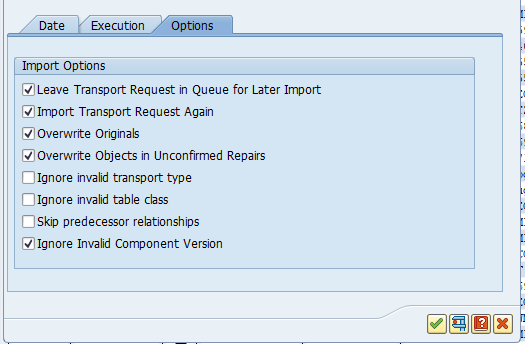
In the below solutions there is reference to the use of these options.
Adding transport again to the import queue
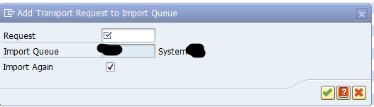
To re-import transport again, go to transaction STMS, go to the import queue, select the menu Extra, Other Requests, Add. Enter the transport request and tick the box Import Again:
Local repair
For some reason the ABAP code was changed locally in the target system.
The text looks like “was repaired in this system”:
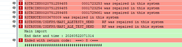
Solution: re-import with the overwrite originals flag, and set the flag overwrite objects in unconfirmed repairs.
Component version mismatch
A very frequent cause of transport errors can be component version mismatch. This means that the system detects a difference in components between the source and target (more on components in this blog). That can be a component (like add on) that is already installed on the source , but not yet on target. Or that in the source the ST-PI or ST-A/PI is already patched, but not on the target.
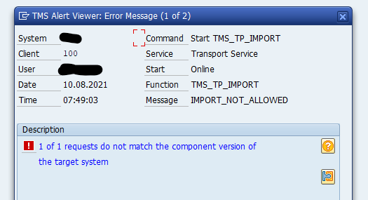
In most cases this version mismatch can be ignored and you can set the “Ignore Invalid Component Version” flag.
When not to set this flag:
- Transports related to newly installed addon like customizing/workbench needing the new component
- Transports with OSS notes related to this component (for example OSS notes on top of ST-PI)
Missing ABAP object references
A very common cause of RC-8 is that an ABAP program needs an object, which the developer stored in a different transport. To fix the RC-8: import first the transport with the object, then the ABAP program transport. Or import them both at the same time.
To avoid such RC-8’s always run the transport sequence check tool, as explained in this blog.