SAP audit log can have high volumes. For that reason most companies use file system to write the audit log.
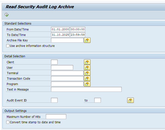
If you have a SIEM (Security Information and Event Management) solution (like SAP enterprise treat detection, Onapsis, SecurityBridge and many more) that needs to scan your audit log, the best way is to store the audit log data in the database. This ensures that the audit log can be analyzed at high performance.
The unfortunate side of storing in the database means that the audit log table can grow quite fast, which is expensive especially if you run on HANA.
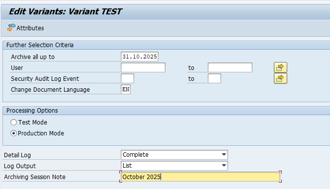
To counter the high costs, you can unload the data from the database into archive files for SAP audit log. This means that your most recent data is in the database for fast analysis, and your history is on cheaper disc storage.
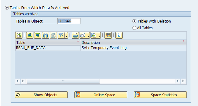
This blog will explain how to archive production order data via object BC_SAL. Generic technical setup must have been executed already, and is explained in this blog.
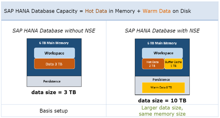
SAP HANA Native Storage Extension (NSE) in a built-in method of SAP HANA, which can be activated and used to offload data to the filesystem, without the need to load it into memory.
The database size can be increased without the need to scale-up or scale-out the database.
All data in the database has a Load Unit property, which defines how data is accessed, loaded and processed by the HANA database.
The data in NSE is “page-loadable”, which means that it is loaded on request by the HANA resource manager into the NSE buffer cache.
The buffer cache manages its own memory pools allocating memory on demand, releasing unused memory and applying smart caching algorithms to avoid redundant I/O operations. A good sizing is important. Too small can lead to Out-Of-Buffer (OOB) events and performance issues. Too large is a waste of memory.
The NSE Advisor is a tool that provides recommendations about load units for tables, partitions or columns. It helps to decide which data should be placed in NSE being page loadable. The required view is “M_CS_NSE_ADVISOR”, which results in a list of tables, partitions and columns with suggestions on whether they should be page or column loadable.
1.1 Reasons
The main reasons for implementing HANA NSE, are:
Reduce HANA memory footprint
Reduce HANA License Costs
Reduce Hardware Costs (no need to Scale-Up or Scale-Out)
1.2 Restrictions
Currently, it is not possible to change the partitioning definition as well as the load unit of a table at once. First, the table needs to be partitioned using the heterogeneous partitioning definition, afterwards, the load unit can be changed for the whole table or individual partitions.
2. Load Units
There are two types of load units:
Column-loadable: columns are fully loaded into memory when they are used.
Page-loadable: columns are not fully loaded into memory, but only the pages containing parts of the column that are relevant for the query.
The load unit can be defined with CREATE or ALTER statements for tables, partitions or columns.
When not specified, it contains the value “DEFAULT”, which is “column loadable”, but it takes over the value from its parent: Table -> Partition -> Column
Example:
Type
Specified Load Unit
Effective Load Unit
Table
DEFAULT
COLUMN
Partition
Page Loadable
Page Loadable
Column
DEFAULT
Page Loadable
3. Identify WARM data
3.1 Static Approach
Based on these characteristics and some knowledge about your applications you can apply a static approach to identify warm data:
Less-frequently accessed data in your application(s) is e.g. application log-data or statistics data. Their records are often written once and rarely read afterwards.
Less-frequently accessed data is also historical data in the application. Some application tables have e.g. a date/time column that provides an indicator to “split” a table in current and older (historical) parts. This table split can be implemented by a table range-partitioning in the HANA database, where the partition key is e.g., the data/time column in your table.
Without too much knowledge about the applications running on the database, you may also monitor the table access statistics in HANA (m_table_statistics or in the SAP HANA Cockpit) to identify rarely accessed tables.
3.2 Dynamic Approach
This can be achieved with the NSE Advisor.
Since S/4HANA 2021 there are over 150 objects delivered during the EU_IMPORT phase from SAP. The most common once are dictionary tables like DD03L, DOKTL, DYNPSOURCE, TADIR etc. This means every customer with S/4 2021+ will now use NSE. So, please take care of your configuration.
4. Implementation
The NSE implementation contains 3 phases:
Pre-checks
Plan
Execute
4.1 Pre-checks
Before starting, it is wise to perform some checks to define the current situation.
The following SQL commands can be executed in the HANA tenant on which the NSE will be activated:
Used memory
select to_decimal(sum(USED_MEMORY_SIZE)/1024/1024/1024,2,2) "Memory Gb" from M_SERVICE_COMPONENT_MEMORY;
Memory size for tables
select to_decimal(sum(MEMORY_SIZE_IN_TOTAL)/1024/1024/1024,2,2) as "MEM_SIZE_GB"from M_CS_TABLES;
Memory size per component
select COMPONENT, to_decimal(sum(USED_MEMORY_SIZE)/1024/1024/1024,2,2) "Memory Gb"from M_SERVICE_COMPONENT_MEMORYgroup by COMPONENTorder by COMPONENT;
Column store size
select to_decimal(sum(PAGE_SIZE*USED_BLOCK_COUNT)/1024/1024/1024,2,2) as "CS Size GB"from M_DATA_VOLUME_PAGE_STATISTICSwhere not PAGE_SIZECLASS like '%-RowStore';
4.2 Plan
This phase consist of determining the objects candidates that can be offloaded. There are a few possible options which can/should be combined to come to a proper offload plan.
These are the possible options:
NSE Advisor
Technical and Dictionary Tables
Tables with a low read count
Partitions with low read count
Statistic Server Tables
Audit Log Tables
Partitioning
4.2.1 NSE Advisor
The NSE advisor should only be used either with the HANA Cockpit or the built-in procedure. A mix of both will lead to wrong results.
Use the advisor for representative workloads of your system.
To limit the CPU consumption of the NSE Advisor, set the following parameters:
min_row_count Exclude objects with less than X rows (default: 10000)
min_object_size Ignore objects smaller than X bytes (default: 1048576)
Note: NSE Advisor Recommendations are NOT persistent over a restart!
4.2.1.1 Enable NSE Advisor
Enable via the HANA Cockpit:
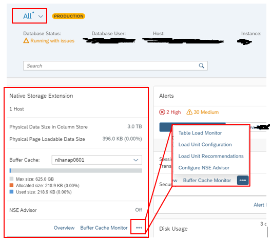
Go to the HANA database, select view “All”. In tile “Native Storage Extension”, click in the three dots and choose “Configure NSE Advisor”:
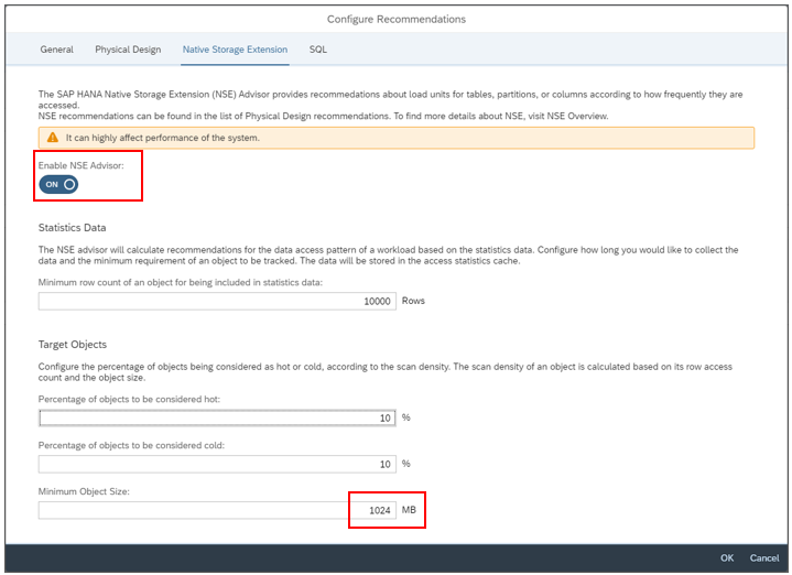
Set the “Enable NSE Advisor” to “ON” and change the “Minimum Object Size” to “1024” MB:
4.2.1.2 Retrieve NSE Advisor recommendations
Generally, the NSE Advisor recommends that you change the load unit of a table, partition, or a column to:
Page-loadable to reduce memory footprint without much performance impact.
Column-loadable to improve performance by keeping hot objects in memory.
The following views can be queried to determine the advices from the NSE Advisor:
M_CS_NSE_ADVISOR
An overview of the objects to be changed:
select * from M_CS_NSE_ADVISOR order by confidence desc;
Same as previous, but in more readable format and only selecting required columns:
select SCHEMA_NAME as SCHEMA, TABLE_NAME, PART_ID, COLUMN_NAME, GRANULARITY as CHANGE_ON, CONFIDENCE,to_decimal(MEMORY_SIZE_IN_MAIN/1024/1024/1024,2,2) as "SIZE_MEM_GB",to_decimal(MAIN_PHYSICAL_SIZE/1024/1024/1024,2,2) as "SIZE_PHYS_GB"from M_CS_NSE_ADVISORwhere not CONFIDENCE = '-1'order by CONFIDENCE desc;
M_CS_NSE_ADVISOR_DETAILS
An overview with more details of all the objects checked:
select * from M_CS_NSE_ADVISOR_DETAILS order by confidence desc;
Same as previous, but in more readable format and only selecting required columns:
select SCHEMA_NAME as SCHEMA, TABLE_NAME, PART_ID, COLUMN_NAME, GRANULARITY as CHANGE_ON,CONFIDENCE, CURRENT_LOAD_UNIT as CHANGE_FROM, TARGET_LOAD_UNIT as CHANGE_TO,to_decimal(MEMORY_SIZE_IN_MAIN/1024/1024/1024,2,2) as "SIZE_MEM_GB",to_decimal(MAIN_PHYSICAL_SIZE/1024/1024/1024,2,2) as "SIZE_PHYS_GB"from M_CS_NSE_ADVISOR_DETAILSwhere not CONFIDENCE = '-1'order by CONFIDENCE desc;
Explanation of the columns:
Column name
Renamed Column
Description
SCHEMA_NAME
SCHEMA
Displays the schema name.
TABLE_NAME
Displays the table name.
COLUMN_NAME
Displays the column name. When the recommendation level is not column, this field is not applicable and the value NULL is used.
PART_ID
Displays the table partition ID. When the recommendation level is not Partition, this field is not applicable, and the value is 0.
CURRENT_LOAD_UNIT
CHANGE_FROM
Displays the current load unit for this object: COLUMN/PAGE.
TARGET_LOAD_UNIT
CHANGE_TO
Displays the recommended load unit for this object: COLUMN/PAGE.
GRANULARITY
CHANGE_ON
Displays the object level at which the recommendation for this table is given: TABLE, PARTITION, or COLUMN.
MEMORY_SIZE_IN_MAIN
SIZE_MEM_GB
Displays the memory consumption size, in bytes, per granularity of the object in main memory. If not LOADED, the value is 0 is used.
MAIN_PHYSICAL_SIZE
SIZE_PHYS_GB
Displays the storage size, in bytes, per granularity of the object.
CONFIDENCE
How sure the NSE advisor is about performing the change.
Note: Columns $trexexternalkey$ or $AWKEY_REFDOC$GJAHR$ are internal columns (SAP Note 2799997 – Q15 “How to handle NSE advisor recommendations to move columns like $trexexternalkey$ or $AWKEY_REFDOC$GJAHR$?”) that refer to the primary key respectively a multi-column index/concat attribute. Indexes can be moved to NSE as well.
Identify index name:
select SCHEMA_NAME, TABLE_NAME, INDEX_NAME, INDEX_TYPE, CONSTRAINT
from INDEXES where TABLE_NAME = '<table_name>';
Change the index load granularity
ALTER INDEX "<schema>"."<index_name>" PAGE LOADABLE;
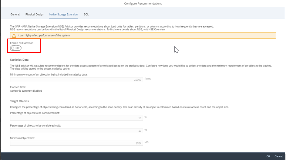
4.2.1.3 Disable the NSE Advisor
In the same screen as the enable function, now set the “Enable NSE Advisor” to “OFF”.
4.2.2 Technical and Dictionary Tables
Some technical and dictionary tables can be offloaded, as they are not read often and only inserts are being performed.
Note: Be careful with CDPOS and CDHDR, as after changing these tables, the NSE advisor gives:
CDHDR should be changed back to COLUMN loadable.
CDPOS should be changed back to COLUMN loadable for columns OBJECTID and CHANGENR
4.2.2.1 Page Preferred versus Page Enforced
Starting SAP S/4HANA 2021, there are tables with ‘paged preferred’ load unit in ABAP Data Dictionary (DDIC):
Run report DD_REPAIR_TABT_DBPROPERTIES for all tables (‘check only’ option) to determine tables having a ABAP DDIC load unit ‘page preferred’ but have actual load unit ‘column’ in the HANA database.
For a quick glance on the load unit settings in DDIC, you may check field LOAD_UNIT in table DD09L:
‘P’= ‘page preferred’, ‘Q’ ‘page enforced’
The following query can be used to determine the table partitions of which the preferred load unit is ‘PAGE’, but the actual load unit is ‘COLUMN’:
select a.SCHEMA_NAME, a.TABNAME, a.LOAD_UNIT, b.LOAD_UNIT, to_decimal(sum(b.MEMORY_SIZE_IN_TOTAL/1024/1024/1024,2,2) "Memory G"from <SAP Schema>.DD09L a, M_CS_TABLES bwhere a.TABNAME = b.TABLE_NAMEand b.LOAD_UNIT = 'COLUMN'and a.LOAD_UNIT = 'P'group by a.TABNAME, a.LOAD_UNIT, b.LOAD_UNITorder by sum(b.MEMORY_SIZE_IN_TOTAL/1024/1024/1024) desc;
The load unit is only applied to the database table (runtime object in SAP HANA) upon creation of the table. As a consequence, if the DDIC setting of an existing table that is initially “column loadable” is changed to “page preferred” in a new release of SAP S/4HANA, an upgrade to that release will not change the load unit setting of the database table – the table will remain “column loadable” in SAP HANA.
Changing from one preferred load unit to another does not change the load unit on the database.
The ABAP DDIC consistency check does not consider the load unit. It is accepted if the load unit on the database differs from the values specified in the DDIC.
During a table conversion, the actual NSE settings of the runtime object in the HANA database will be preserved.
Column Enforced or Page Enforced
The load unit is specified upon creation of the table. Furthermore, changes to the load unit in the ABAP DDIC result in corresponding changes on the database.
Changing the enforced load unit results in a corresponding change on the database.
The ABAP DDIC consistency check takes the load unit into account. Different values for the load unit in the DDIC and on the database result in tables that are inconsistent from the DDIC point of view.
For the “Page Enforced” load unit setting, the technical restrictions apply as described in the context of S/4HANA 2020.
For the “Enforced” flavor of load unit settings, the behavior during table conversion is as described in the context of S/4HANA 2020.
4.2.3 Statistics Server Tables
The ESS (embedded statistics server) tables are not part your business workload. They are used for the performance and workload data of the system. This means they are only used for read load when you have some issues and your DBA or SAP is analyzing the system. These column tables of the SAP HANA statistics server are not using NSE as default. It is recommended to also activate NSE for the column tables of the SAP HANA statistics server.
Determine the current load unit:
select distinct LOAD_UNIT from SYS.TABLES where SCHEMA_NAME = '_SYS_STATISTICS' and IS_COLUMN_TABLE = 'TRUE' and IS_USER_DEFINED_TYPE = 'FALSE';
When the output value is ‘DEFAULT’, activate NSE for column tables of HANA statistics server using PAGE LOADABLE by running the following command with a user with sufficient permissions:
call _SYS_STATISTICS.SHARED_ALTER_PAGE_LOADABLE;
4.2.6 Audit Log Tables
Starting with HANA 2.0 Rev. 70 it is possible to page out the table “CS_AUDIT_LOG_”.
Check the current setting with the following command:
select LOAD_UNIT from SYS.TABLES where SCHEMA_NAME = '_SYS_AUDIT' and TABLE_NAME = 'CS_AUDIT_LOG_';
When the output value is ‘DEFAULT’, activate NSE for the audit log tables with the following command:
ALTER SYSTEM ALTER AUDIT LOG PAGE LOADABLE;
4.2.7 Partitioning
When NSE is used for a table (regardless of whether the full table is page loadable, or only selected columns or partitions), comparatively small partitions should be designed in order to optimize IO-intensive operations such as delta merges. Because of the focus on IO, the relevant measurable is not the number of records per partition, but rather the partition size in bytes. When using NSE with a table, partition sizes should be smaller than 10 GB. This also means that if the size of a table that is fully or partially (selected columns) in NSE reaches 10 GB, this table should be partitioned.
This should be analyzed and tested carefully and depends highly on the usage of the table by your business. Mostly the current and the last year is interesting for most scenarios. This means anything older than 2 years can be paged out. Here you have to choose a partition attribute. Mostly there is a time range attribute like FYEAR or GJAHR. Here you can partition by year / quarter / month. This depends on the amount of data.
Monitoring the buffer hit ratio, fill degree of partitions, performance of SQLs (may be new coding which was not analyzed) and creating new partitions for new months, quarter or years. It is an ongoing process and every new HANA revisions has its own new features.
The following query retrieves partitioned tables with range partitions older than 3 years.
select a.schema_name, a.table_name, c.part_id, replace(b.LEVEL_1_EXPRESSION,'"','') "Column",
max(c.LEVEL_1_RANGE_MIN_VALUE) "Last_Range_From",
max(c.LEVEL_1_RANGE_MAX_VALUE) "Last_Range_To",
to_decimal(d.memory_size_in_total/1024/1024/1024,2,2) as "MEM_SIZE_GB", to_decimal(d.disk_size/1024/1024/1024,2,2) as "DISK_SIZE_GB"
from m_tables a, partitioned_tables b, table_partitions c, m_table_partitions d
where a.IS_COLUMN_TABLE = 'TRUE'
and a.is_partitioned = 'TRUE'
and b.level_1_type = 'RANGE'
and a.table_name = b.table_name
and b.table_name = c.table_name
and c.table_name = d.table_name
and c.part_id = d.part_id
and d.load_unit <> 'PAGE'
and b.LEVEL_1_COUNT > 1
and c.LEVEL_1_RANGE_MAX_VALUE < add_years(current_timestamp,-4)
and not c.LEVEL_1_RANGE_MAX_VALUE = ''
group by a.schema_name, a.table_name, b.LEVEL_1_EXPRESSION, b.LEVEL_1_COUNT, c.part_id, to_decimal(d.memory_size_in_total/1024/1024/1024,2,2), to_decimal(d.disk_size/1024/1024/1024,2,2)order by a.table_name, c.part_id;
Explicitly specifies the upper limit of the buffer cache, in MBs.
max_size_rel
% of GAL
Specifies the upper limit of the buffer cache as a percentage of the global allocation limit (GAL) or the service allocation limit if set.
unload_threshold
80% of max_size
Specifies the percentage of the buffer cache’s maximum size to which it should be reduced automatically when buffer capacity is not fully used. 80% is a good starting value.
Note: When both max_size and max_size_rel are set, the system uses the smallest value. When applying the values to a scale-out system at the DATABASE layer, max_size_rel will be relative to the allocation for each host, which can be different for each.
SQL Commands to be performed in the SYSTEMDB:
ALTER SYSTEM ALTER CONFIGURATION ('global.ini','SYSTEM') SET ('buffer_cache_cs','max_size') = '<size_in_MB>' WITH RECONFIGURE;
ALTER SYSTEM ALTER CONFIGURATION ('global.ini','SYSTEM') SET ('buffer_cache_cs','max_size_rel') = '10' WITH RECONFIGURE;
ALTER SYSTEM ALTER CONFIGURATION ('global.ini','SYSTEM') SET ('buffer_cache_cs','unload_threshold') = '80' WITH RECONFIGURE;
4.3.2 Add objects to NSE
For the identified objects (tables, columns, indexes, partitions), you can change the load unit to the required value with the following commands:
Table ALTER TABLE <TABLE_NAME><TYPE> LOADABLE;
Index ALTER INDEX <INDEX_NAME><TYPE> LOADABLE;
Column ALTER TABLE <TABLE_NAME> ALTER (<COLUMN> ALTER <TYPE> LOADABLE);
Partition ALTER TABLE <TABLE_NAME> ALTER PARTITION <PARTITION_ID><TYPE> LOADABLE;
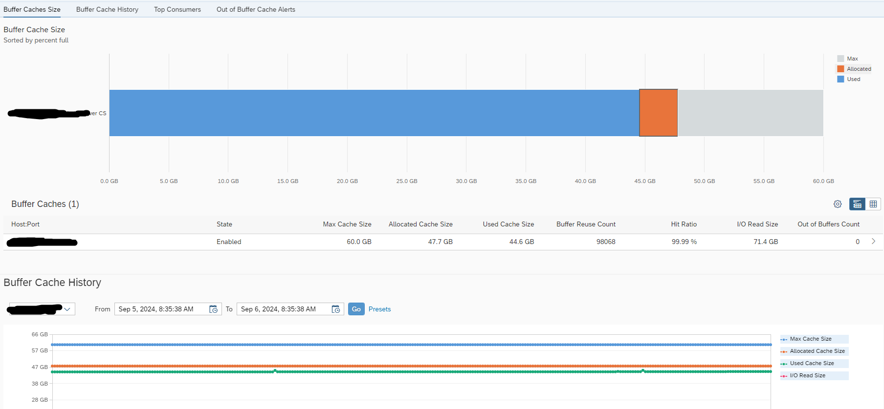
4.3.3 Monitoring the Buffer Cache
4.3.3.1 HANA Cockpit
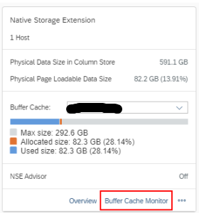
The buffer cache can be monitored from the HANA Cockpit tile “Native Storage Extension”.
4.3.3.2 SQL Commands
Also the following views can be queried:
HOST_BUFFER_CACHE_STATISTICS
HOST_BUFFER_CACHE_POOL_STATISTICS
4.3.3.2.1 NSE Buffer Cache Usage
The following query can be used to determine the current usage of the NSE Buffer Cache. The “Used%” should be below 80:
select to_decimal((sum(USED_SIZE)/1024/1024/1024) / (avg(MAX_SIZE)/1024/1024/1024) * 100,2,2) "Used %"
from M_BUFFER_CACHE_STATISTICS
where CACHE_NAME = 'CS'
group by CACHE_NAME;
4.3.3.3.2 NSE Buffer Cache Hit Ratio
The following query can be used to determine the Hit Ratio of the NSE Buffer Cache. The “Hit Ratio %” should be above 90:
select to_decimal(avg(HIT_RATIO),2,2) "HIT_RATIO %" from M_BUFFER_CACHE_STATISTICS
where CACHE_NAME = 'CS'
and not HIT_RATIO = 0
group by CACHE_NAME;
4.3.3.4.3 Max. NSE Buffer Cache Size
The following query can be used to determine the maximum possible size of the NSE Buffer Cache, based on the current offloaded objects:
select to_decimal(sum("Size_in_GB")/1024/1024/1024,2,2) "Size_in_GB"
from
(select sum(ESTIMATED_MAX_MEMORY_SIZE_IN_TOTAL) "Size_in_GB"
from M_CS_TABLES
where LOAD_UNIT = 'PAGE'
union
select sum(UNCOMPRESSED_SIZE) "Size_in_GB"
from M_CS_COLUMNS
where LOAD_UNIT = 'PAGE'
and not TABLE_NAME in (select TABLE_NAME from M_CS_TABLES where LOAD_UNIT = 'PAGE')
union
select sum(INDEX_SIZE) "Size_in_GB"
from M_RS_INDEXES
union
select sum(MEMORY_SIZE_IN_TOTAL) "Size_in_GB"
from M_TABLE_PARTITIONS
where LOAD_UNIT = 'PAGE'
and not TABLE_NAME in (select TABLE_NAME from M_CS_TABLES where LOAD_UNIT = 'PAGE'));
4.3.3.4.4 NSE Buffer Cache Max. Size vs Configured Size
The following query can be used to determine the maximum possible size of the NSE Buffer Cache, based on the current offloaded objects versus the configured size.
The “Max vs Conf %” should be lower than 100:
select to_decimal((sum(a."Size_in_GB")/b."Max_GB")*100,2,0) as "Max_vs_Conf %"
from
(select sum(ESTIMATED_MAX_MEMORY_SIZE_IN_TOTAL) "Size_in_GB"
from M_CS_TABLES
where LOAD_UNIT = 'PAGE'
union
select sum(UNCOMPRESSED_SIZE) "Size_in_GB"
from M_CS_COLUMNS
where LOAD_UNIT = 'PAGE'
and not TABLE_NAME in (select TABLE_NAME from M_CS_TABLES where LOAD_UNIT = 'PAGE')
union
select sum(INDEX_SIZE) "Size_in_GB"
from M_RS_INDEXES
union
select sum(MEMORY_SIZE_IN_TOTAL) "Size_in_GB"
from M_TABLE_PARTITIONS
where LOAD_UNIT = 'PAGE'
and not TABLE_NAME in (select TABLE_NAME from M_CS_TABLES where LOAD_UNIT = 'PAGE')) a,
(select top 1 MAX_SIZE "Max_GB"
from _SYS_STATISTICS.HOST_BUFFER_CACHE_STATISTICS
order by SERVER_TIMESTAMP desc) b
group by b."Max_GB";
4.3.3.3 SAP Focused Run monitoring
Active monitoring of the buffer cache can also be implemented using SAP Focused Run.
The metrics should be configured for each HANA tenant database, in System Monitoring / Performance / Database Performance.
The following metrics are being monitored.
NSE Buffer Cache Metric
Yellow
Red
SQL Reference
Usage
> 80
> 90
See NSE Buffer Cache Usage
Hit Ratio
< 95
< 90
See NSE Buffer Cache Hit Ratio
Max. Size vs Configured Size
>= 98
>= 100
See NSE Buffer Cache Max. Size vs Configured Size
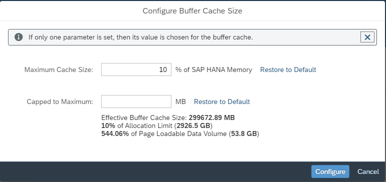
4.3.4 Edit NSE Buffer Cache
If the NSE Buffer Cache should be resized, based on the analysis above, calculate the required size in MB.
In the HANA Cockpit this can be changed in the Buffer Cache Monitor screen, by clicking on the button “Configure Buffer Cache Size”:
Set the required values (in MB) and click “Configure”:
This can also be changed with an SQL command: (Change the <size_in_MB> to the correct value)
ALTER SYSTEM ALTER CONFIGURATION ('global.ini','SYSTEM') SET ('buffer_cache_cs','max_size') = '<size_in_MB>' WITH RECONFIGURE;
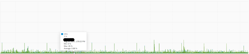
5. Performance impact
5.2 NSE Advisor
The NSE Advisor, in theory, cause an overhead on the database, however in practice we haven’t noticed a significant increase in CPU/Memory Consumption.
5.2 NSE Buffer Cache
NSE Buffer Cache sizing is an important and regular exercise.
Configuring a too large buffer cache size that would avoid any disk I/O, but also keep too many and rarely accessed warm data in memory, would lead to the best performance, but inefficient buffer cache size. If that required, it would be better to keep all data as column loadable (no NSE usage)
Configuring a too small buffer cache size where the requested warm data cannot be loaded into memory (leads to query cancellation, i. e. Out-of-Buffer event). Or, the disk I/O for warm-data processing causes an unacceptable query performance which might even affect the decrease of the overall system performance of HANA.
Note: It is not recommended to aggressively define a very low percentage to enforce the buffer cache to release allocated memory. It may lead to the situation where the buffer cache needs to allocate memory immediately after releasing that memory. The de-allocation and re-allocation of memory brings a lot of overhead and performance degradation in NSE.
6. Required Permissions
Analysis can be done with your personal user-id. But do set up the required HANA roles and permissions.
7. Periodic Tasks
The following tasks have to be performed regularly (at least every 6 months):
Monitoring
Check out-of-buffer events
Run NSE advisor
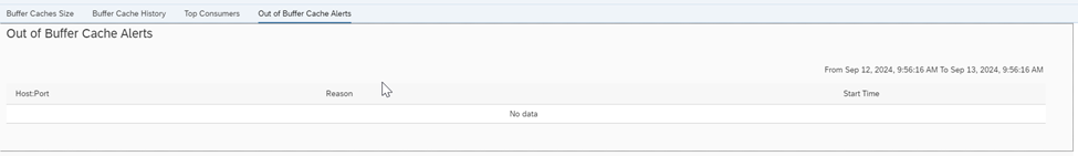
7.1 Check Out-Of-Buffer Events
When your buffer cache is not large enough to handle your workload, SAP HANA generates an alert message.
During an out-of-buffer situation, regular user tasks may be rolled back, and critical tasks (for example, recovery) use the emergency buffer pool.
Checking the OOB-events can be performed via the HANA Cockpit, in tile NSE, choose “Buffer Cache Monitor” and select tab “Out of Buffer Events”.
For each out of buffer entry, the following information is provided:
Column
Description
Host/Port
Specifies the host name and internal port of the HANA service.
Type
Specifies the type of the event.
Reason
Specifies additional information for the event (for example, the number of buffer cache used and how many buffer cache are needed).
Creation Time
Specifies the time the event occurred.
Update Time
Specifies the time the event was last updated.
Handle Time
Specifies the time a user performed an operation that resolved or alleviated the issue related to the event.
State
Specifies the current state of the event (for example, NEW, HANADLED).
Determine the reason why these OOB-events happened. This can have several causes:
Reason
Possible Solution(s)
Buffer cache size too low
Increase the NSE Buffer Cache
Objects being accessed too frequently
Change the load attribute, to put them into main memory again
Partition the table and determine which partitions should be put to NSE
7.3 Run NSE Advisor
Activate the NSE Advisor once every 6 months, during as respective workload, to review the current NSE settings.
This might give an indication that tables have to be added to the main memory again and/or that additional tables can be offloaded to the NSE.
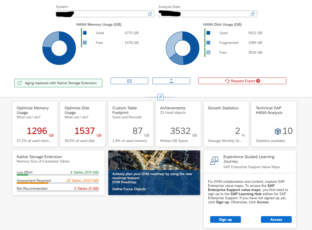
On the start screen it is important to first select the System and Analysis Date.
The top part:
The top part contains overview for database size.
Then there are tiles to start working on:
Optimize memory usage
Optimize disk usage
Custom table footprint
Achievements
Growth statistics
Technical HANA analysis
Use of NSE (native storage extension)
Link to the DVM roadmap function
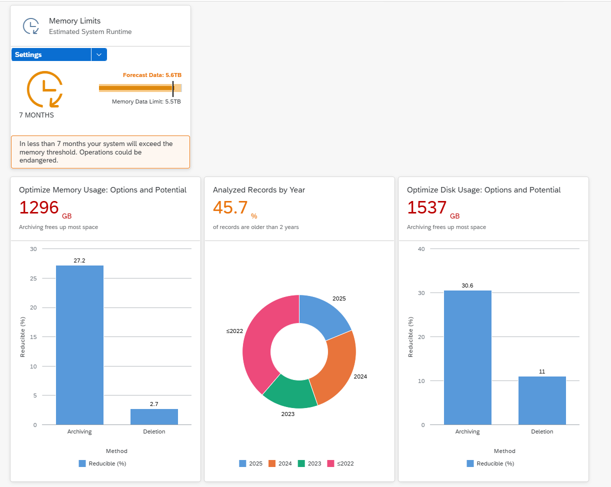
If you scroll down to the bottom part:
Here you find tiles that can help you on:
Memory limits
Optimize memory usage
Record analysis per year
Optimize disc usage
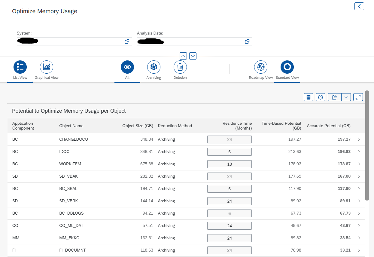
Use case 1: finding objects for archiving and/or deletion
In the first tile “Optimize memory usage” you can get details on potential objects to archive and delete:
SAP uses a default archiving retention period which is quite aggressive. Please be aware your business might be more conservative.
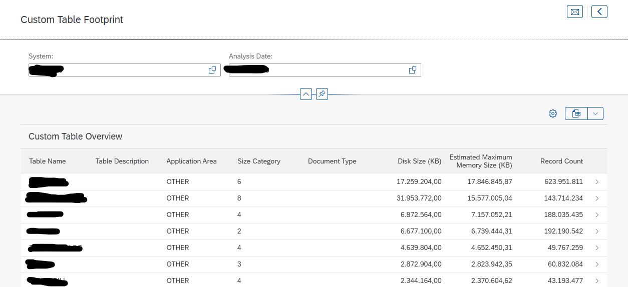
Use case 2: custom table footprint
The main tile for custom table footprint already indicates the % of table size that is for custom tables.
Inside the tile you can see which table is larger and/or is having many entries:
For custom tables you can consider writing dedicated clean up programs.
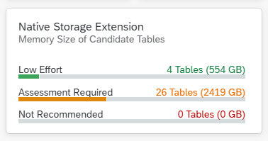
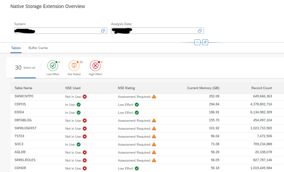
Use case 3: check effectiveness of your NSE setup
You can use the NSE tile to check the effectiveness of your NSE (native storage extension) setup (follow this link to blog on NSE explanation). And you can see if more object might be eligible for NSE.
This blog will explain how to archive production order data via object PP_ORDER. Generic technical setup must have been executed already, and is explained in this blog.
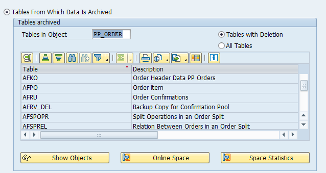
Object PP_ORDER
Go to transaction SARA and select object PP_ORDER.
Dependency schedule is empty, so there are no dependencies:
Guided procedure on production order archiving issues can be found here.
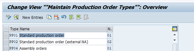
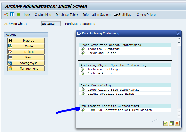
Application specific customizing
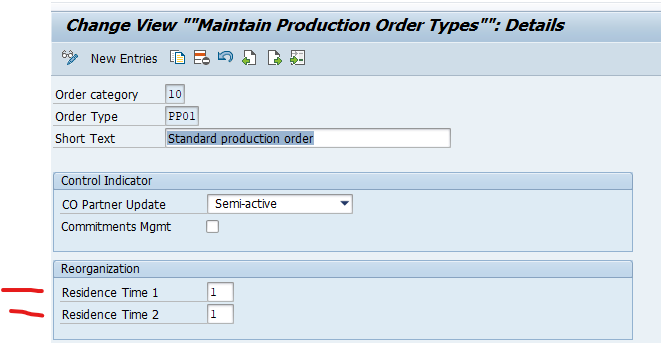
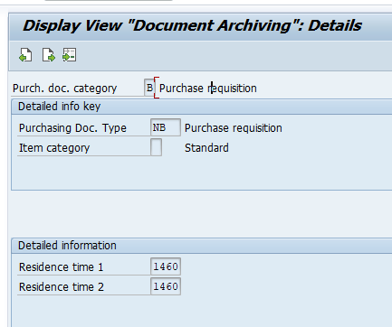
For archiving object PP_ORDER there is application specific customizing to perform. Select the order type:
And set the residence times:
Residence time 1 determines the time interval (in calendar months) that must elapse between setting the delete flag (step 1) and setting the deletion indicator (step 2).
Residence time 2 determines the time (in calendar months) that must elapse between setting the deletion indicator (step 2) and reorganizing the object (step 3).
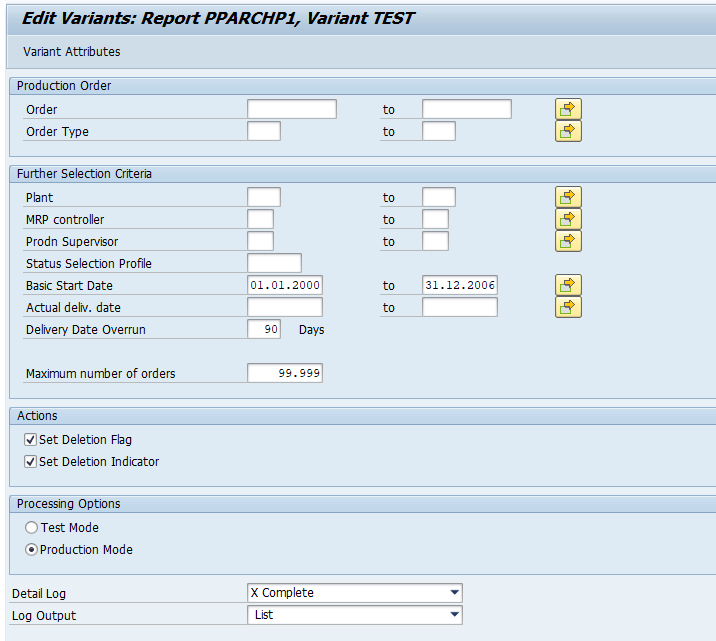
Executing the preprocessing run
In transaction SARA, PP_ORDER select the preprocessing run:
Select your data, save the variant and start the archiving preprocessing run.
The run will show several functional issues: orders that are not completed and could not be marked for deletion with the functional reason.
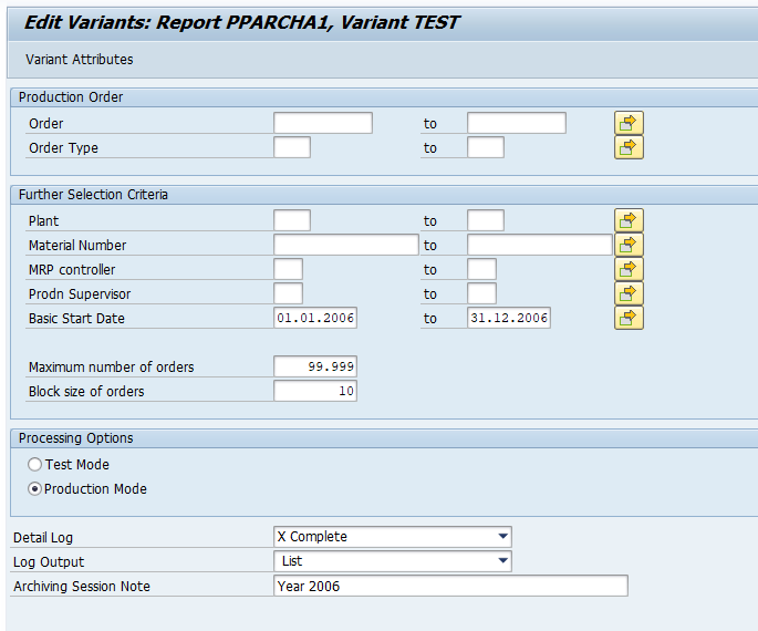
Executing the write run and delete run
In transaction SARA, PP_ORDER select the write run:
Select your data, save the variant and start the archiving write run.
After the write run is done, check the logs. PP_ORDER archiving has low speed, and medium percentage of archiving (60 to 80%).
Proved a good name for the archive file for later use!
Deletion run is standard by selecting the archive file and starting the deletion run.
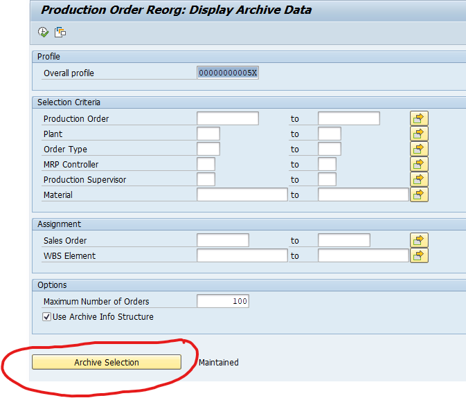
Data retrieval
Data retrieval is via program PPARCHR1:
Important here to select the correct archive files.
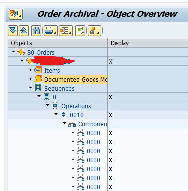
Output is a list on the left side with details on the right hand side of the screen in table format:
This blog will explain how to archive handling units via object LE_HU. Generic technical setup must have been executed already, and is explained in this blog.
Object LE_HU
Go to transaction SARA and select object LE_HU.
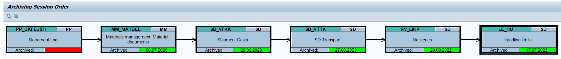
Dependency schedule:
In case you use production planning backflush, you must archive those first. Then material documents, shipment costs (if in use), SD transport (if in use) and deliveries.
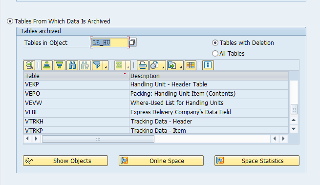
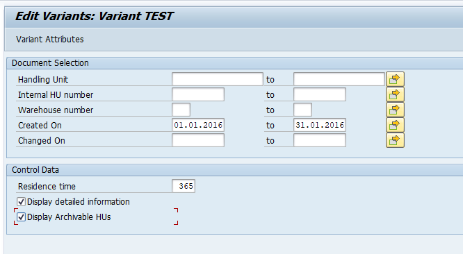
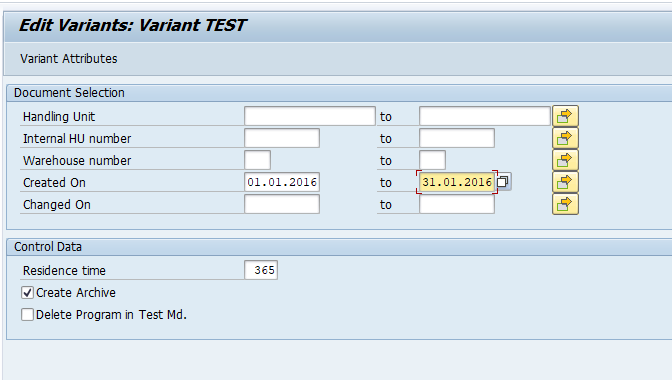
Archiving object LE_HU has no specific customizing. Retention period is set on the write program screen.
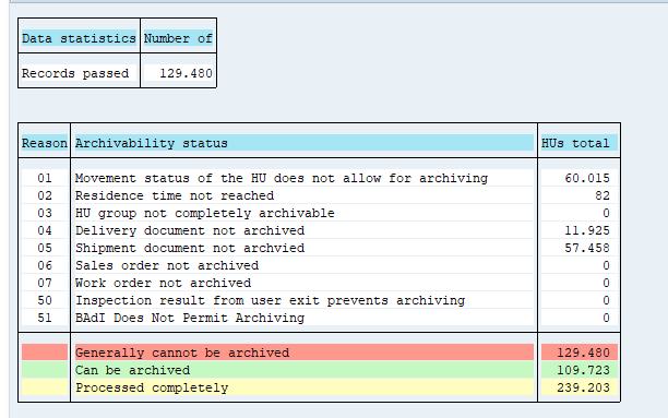
Execution the preprocessing run
In transaction SARA, LE_HU select the preprocessing run:
The run will show you how many can be archived and how many cannot be archived (mainly due to status and preceding documents):
Executing the write run and delete run
In transaction SARA, LE_HU select the write run:
Select your data, save the variant and start the archiving write run.
After the write run is done, check the logs. LE_HU archiving has average speed, but not so high percentage of archiving (about 40 to 90%).
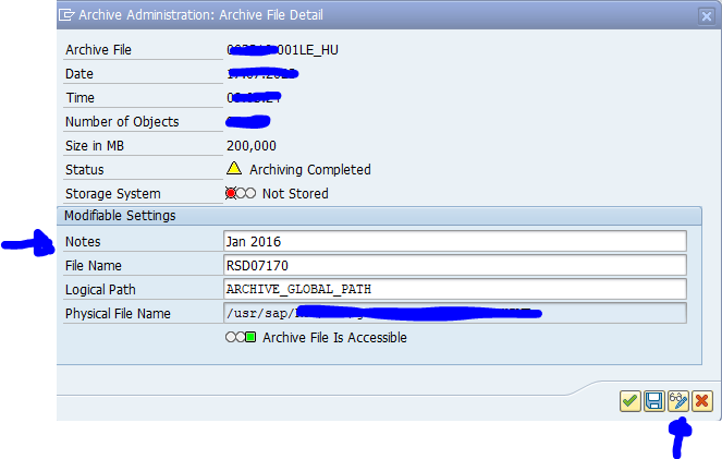
Unfortunately the LE_HU object does not have a Note field to give the archive file a correct name. If you still want to do so, you have to do this in SARA via the management of archiving sessions: select the session and change the description there:
Deletion run is standard by selecting the archive file and starting the deletion run.
Data retrieval
Data retrieval is via program RHU_AR_READ_FROM_ARCHIVE.
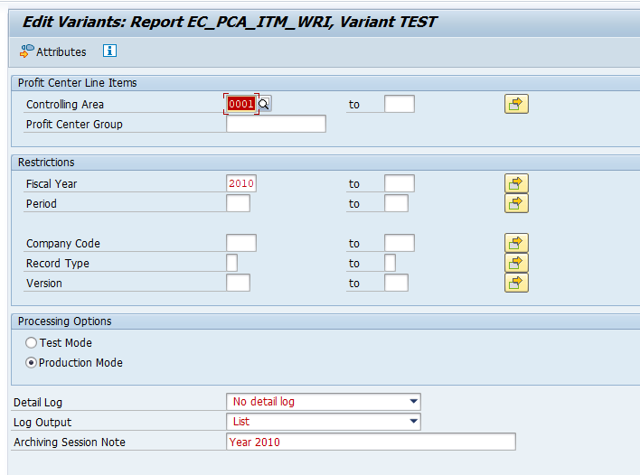
This blog will explain how to archive profit center accounting documents transports via object EC_PCA_ITM. Generic technical setup must have been executed already, and is explained in this blog.
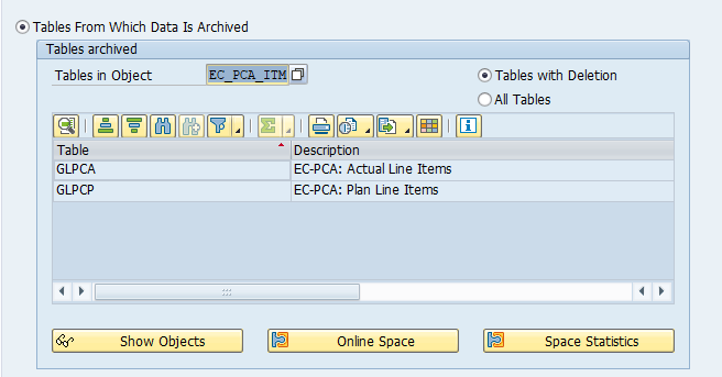
Object EC_PCA_ITM
Go to transaction SARA and select object EC_PCA_ITM.
Dependency schedule:
This means for profit center accounting archiving that there are no dependent objects.
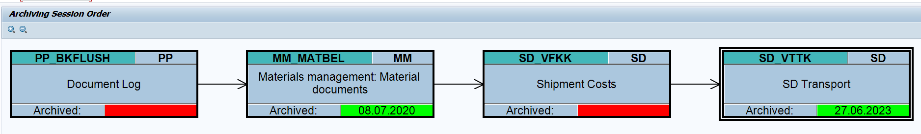
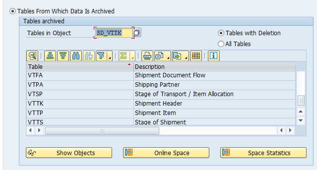
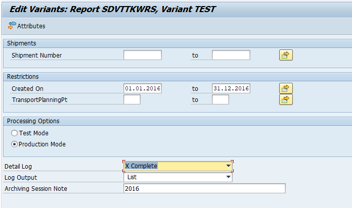
This blog will explain how to archive SD transports via object SD_VTTK. Generic technical setup must have been executed already, and is explained in this blog.
Object SD_VTTK
Go to transaction SARA and select object SD_VTTK.
Dependency schedule:
In case you use production planning backflush, you must archive those first. Then material documents and shipment costs (if in use).
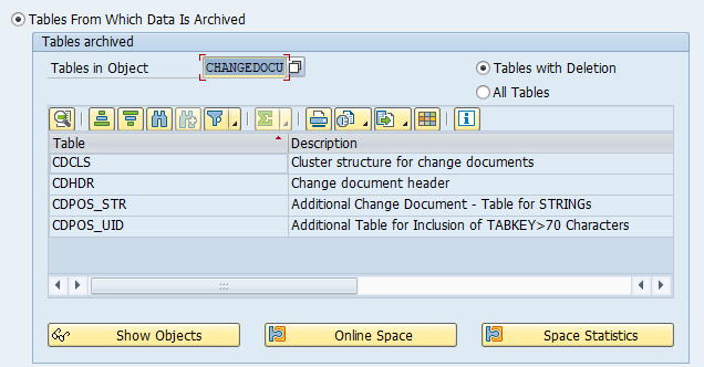
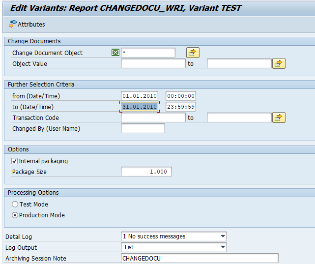
This blog will explain how to archive change documents via object CHANGEDOCU. Generic technical setup must have been executed already, and is explained in this blog.
Object CHANGEDOCU
Go to transaction SARA and select object CHANGEDOCU.
Dependency schedule: (none):
Change documents are archived as part of other archiving objects. For specific changes you might want to archive the changes sooner to get a grip on CDHDR and CDCLS/CDPOS table sizes and amount of entries.
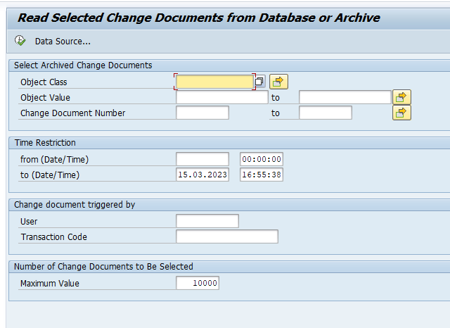
In the second screen select the archive files. Now wait long time before data is shown.
For faster retrieval, setup data archiving infostructures SAP_CHANGEDOCU1 and SAP_CHANGEDOCU2. These are not active by default. So you have to use transaction SARJ to set them up and later fill the structures (see blog).
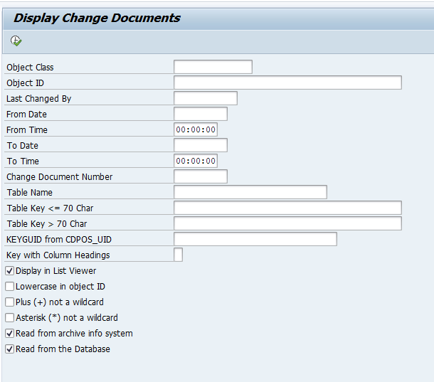
Now transaction RSSCD100 can be use for data retrieval:
Don’t forget to select the tick box “Read from archive info system”.
Another option is via transaction SARE (archive explorer) and then choose object CHANGEDOCU with archive structure SAP_CHANGEDOCU1.
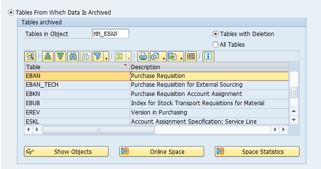
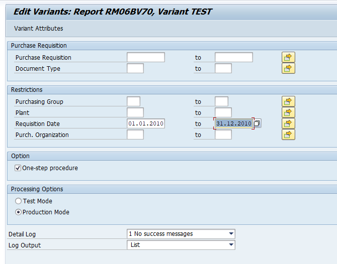
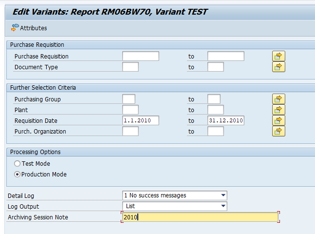
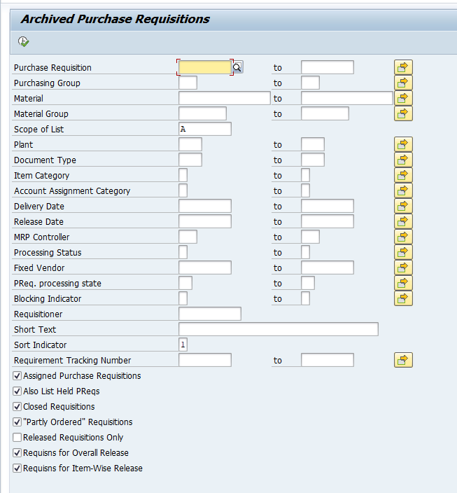
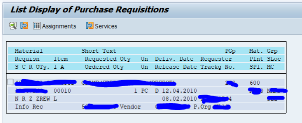
This blog will explain how to archive purchase requisitions via object MM_EBAN. Generic technical setup must have been executed already, and is explained in this blog.
This blog will explain how to archive CATS time writing data via object CATS_DATA. Generic technical setup must have been executed already, and is explained in this blog.
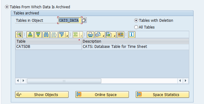
Object CATS_DATA
Go to transaction SARA and select object CATS_DATA.
In the application specific customizing for CATS_DATA is not required.
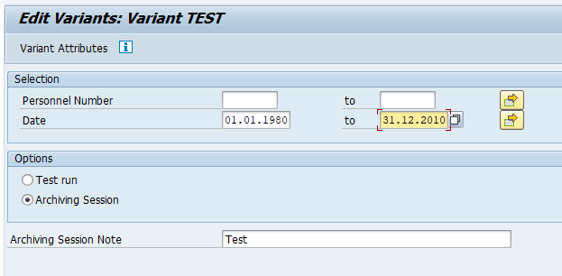
Executing the write run and delete run
In transaction SARA, CATS_DATA select the write run:
Select your data, save the variant and start the archiving write run.
Give the archive session a good name that describes date range. This is needed for data retrieval later on.
After the write run is done, check the logs. CATS_DB archiving has average speed, but high percentage of archiving (up to 100%). Only status 30 (approved) and status 60 (cancelled) are archived. See SAP Help.
Deletion run is standard by selecting the archive file and starting the deletion run.
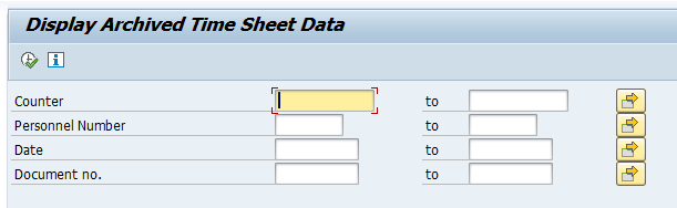
Data retrieval
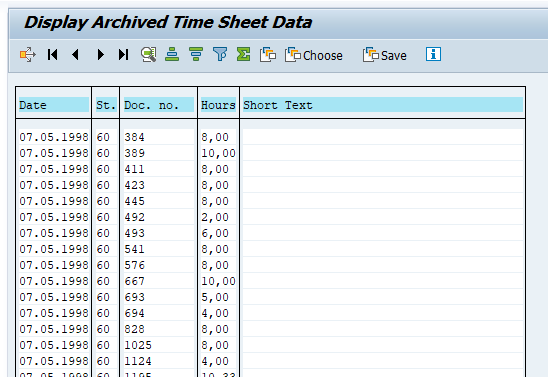
Start the data retrieval program and fill selection criteria:
Result is a simple list:
Data reload program
For emergency cases, there is an undocumented reload program: RCATS_ARCH_RELOADING. Use at own risk.